Project 2 — Hopfield Net
Data structures
You will need a structure to hold the patterns (each with 100
neurons), a 50x100 array will work. A 100x100 array can be used to
store the weights of the network. You will want to represent the
neural network itself, such as with a 100 element array. You will
also want data structures to keep track of the number of stable
imprints and probability of stable imprints, and possibly similar
structures for storing the averages over multiple runs. Arrays of 50
elements can work for this. For the 527 part, you will want to keep
track of the number and frequencies of the basin sizes with
something like a 50x50 array.
Basic code structure
The overall logical flow for main() should be
something like this:
initialize data structures for keeping statistics
for i from 0 to number of runs
  generatePatterns()
  for p from 1 to 50
    imprintPatterns(p)
    testPatterns(p)
compute averages over number of runs
normalize data for basins of attraction (527 students)
write data file
generatePatterns()
Randomly initialize 50 vectors, each with 100 elements, where each
element is 1 or -1. Be sure to seed the random generator in main()
with srand(time(NULL)); or equivalent in your chosen
programming language.
imprintPatterns(p)
This is where you compute the various weights associated with the
neurons, which you will use to calculate the net input (local field)
in a later step. The formula for computing the weights is given by:
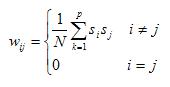
This will calculate the weight associated with neurons i and
j, where i and j each range from 1 to 100 (or
0 to 99, depending on your array indexing scheme). So each weight
represents a pair of neurons. This implies you will have a 100x100
array of weights, as mentioned above.
Start by iterating through i and j. Then if i
and j are not equal (i.e., you have two different neurons),
do the following. Have index k loop through each of the
patterns 1 through p (the parameter passed in). The si
and sj in the above formula represent the state values (1
or -1) for neurons i and j, respectively, for
pattern k. So you will take the product of the state values
of neurons i and j for pattern k, and
accumulate the sum of these products over the p imprinted
patterns (in the k loop). After accumulating the sum, divide
this sum by the number of neurons N (100 in our case). If i
and j are equal, then assign the corresponding weight to 0.
This is what is meant by no self-coupling, a neuron does not have a
weight associated with itself.
So the first time imprintPatterns(p) is called from main(),
it will imprint pattern 1. The next time it is called, it will
imprint patterns 1 and 2. The third time it is called, it will
imprint patterns 1, 2, and 3, and so on. This is how the inner k
loop iterates through the p patterns.
testPatterns(p)
Here is where you will determine the number and fraction of imprints
that are stable (or unstable). First, iterate k from 1
to p (the parameter passed in), and inside that for
loop, do the following:
a. Set the neural net (100 element array) to the current pattern k
by simply copying the array elements over.
b. For each of the 100 neurons (for loop and formula index i)
in the neural net that you just set in the previous step, first
compute its new state value using the following formulas:
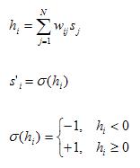
The first formula computes the local field of the neuron. The
variable j iterates through each neuron of the neural net
(100 element array), and multiplies the neuron's state value with
its associated weight matrix value. The variable i
represents the current neuron being considered at the beginning of
step b), so we are interested in row i of the weight matrix.
Keep accumulating this sum of products over the neural net to
compute the local field of the neuron of interest.
The other two formulas determine the next state of the current
neuron, -1 if its local field h is negative, and +1 if its
local field h is nonnegative.
After getting the neuron's new state, compare it to the neuron's
current state (the corresponding value you assigned to the neural
net in step a).
If any of the 100 elements of the neural net differ from its
corresponding new state value, then that imprinted pattern that was
assigned to the neural net is NOT stable. Otherwise, if each element
matches its new state based on the local field computation, then
that imprinted pattern IS stable. You will probably want a boolean
to keep track of whether or not the current imprinted pattern is
stable.
Note: all of the items in this step b) are contained in a loop that
iterates through the 100 elements of the neural net.
c. If the pattern is stable, increment a counter indicating the
number of stable patterns for the current p. You can use an
array of 50 elements for this (one for each p).
d. To compute the probability of stable imprints for each p,
divide the number of stable imprints for that p by
that number p. To get the probability of UNstable imprints
for that p, subtract the probability of stable imprints for
that p from 1. Note that probabilities should never be
greater than 1. Also, the number of stable (or unstable) imprints
for any value of p should never be greater than p
itself.
Graphing the data
You should generate the following two graphs:
a. The fraction of unstable imprints as a function of the number of
imprints (p=1 to 50)

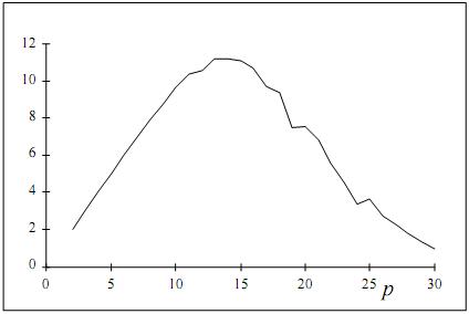
b. The number of stable imprints as a function of the number of
imprints (p=1 to 50)
You can just write the data to a .csv file, and then use a program
like Excel to create the graphs. Your program does not have to
produce the graphs themselves, just the data for the graphs. The
data will consist of the number p, the number of stable
imprints for that p, and the fraction of unstable imprints
for that p. Again, p ranges from 1 to 50.
Repeat the generatePatterns(), imprintPatterns(p),
and testPatterns(p) steps several times, each time
testing a different set of 50 random patterns (vectors). Average
your data over all of these iterations. The more iterations (runs)
you do, the smoother your graphs should look.
Basins of attraction (527 students):
In addition to the undergrad work above, estimate the size of the
basins of attraction for each imprinted pattern for the number of
imprinted patterns p. In part c) in the section testPatterns(p)
above where you test for stability of each of the p
imprinted patterns, add the following:
1. If the pattern is unstable, set its basin size to 0. In
other words, increment the histogram count for basin size 0 for the
current value of p.
2. If the pattern is stable, do:
After incrementing the number of stable patterns for the current
value of p, iterate through the number of permutations that
you want to try (e.g., 5). In this loop, do the following:
a. Generate a permutation of the numbers 1 to 100 by creating an
array of the numbers 1 to 100 (or 0 to 99) in random order. This
list of numbers will indicate which bits of the pattern to flip and
in which order to flip them. You will only need to consider the
first 50 elements of this permutation since the maximum basin size
is 50.
b. Letting j be the loop variable, go through each of the
first 50 elements in the permutation array and:
i. Initialize the neural network to the current pattern k of
the p imprinted patterns.
ii. Flip the states of the positions of the neural network given by
the first j permutation array elements. That is, change a 1
to a -1 and a -1 to a 1 in these j positions of the neural
network. Note that these j positions that you will flip will
not necessarily be the actual first j positions in the
network.
iii. Go through 10 iterations of updating the neural network. Change
each network element according to sigma of its local field h.
Update the network elements in random order. For any of the
iterations, if none of the neurons change from their previous state,
then break from the iterations of updating the neural network.
iv. Check to see if the network is equal to the current imprinted
pattern k after these 10 iterations. If the network is
different than the imprinted pattern k, then break from the
50 iterations of the permutation array. Otherwise, keep going
through the permutation array.
c. The first iteration of the permutation array (as given by j)
where the network does not converge to the current imprinted pattern
k is the number that estimates the size of the basin of
attraction for that imprinted pattern. It is equivalent to the
number of bits in the pattern you need to flip until the network
does not converge to that pattern. If the network converges for all
50 iterations of the permutation array (that is, it never does not
converge), then the size of the basin of attraction for that pattern
is 50, since that is the maximum size of a basin of attraction.
Try the above a-c for several different permutations (say, 5) and
average the results.
3. Increment the counter of the histogram array keeping track of
the basin sizes. You might have a two dimensional array where
the first dimension indicates the number of imprinted patterns
(given by p), and the second dimension gives the size of the
basin of attraction. The actual array element is the count (or
frequency) of that basin size for that p. This will keep
track of a histogram of basin sizes for each value p.
4. Produce a graph of the histograms for various values of p
(even values of p should be enough) as in the following:
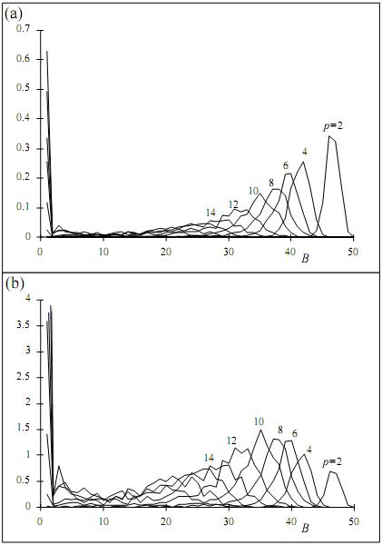
Including the first of the two graphs is enough, but including both
may boost your grade slightly. The first graph is normalized (i.e.,
in terms of frequencies of basin sizes), and the second graph is in
terms of counts of basin sizes. For normalizing the data, keep in
mind the number of permutations you try, the number of different
sets of 50 patterns (i.e., number of runs) you try, and the number
of imprinted patterns p.
Extra credit
The following items will boost your grade slightly or significantly.
- Try different numbers of patterns besides 50, such as 100,
200, etc.
- Try different numbers of neurons besides 100, such as 50, 200,
etc.
- More runs to get smoother graphs.
- Different ways of plotting and analyzing data.
- More in depth analysis and discussion.
- For basins of attraction, graph odd values of p.
- Include both kinds of basins of attraction graphs.
- Implement pseudo-temperature (noise), as described in the
handout.
What to submit
- Report (in .pdf format): This includes your graphs and
your discussion and analysis.
- Source code
Tar or zip your files together and send them to the TA. The
directory should include your report (in .pdf) and your code.