ECE 202: Circuits II

Parameter Sweeps in LTSpice
Parameter sweeps can be a useful tool to examine how circuit operation changes with variation in different passive values, source amplitudes, operating frequency, or any other parameter. To examine how to do a parameter sweep, we will consider a simple R-C circuit:
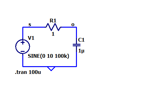
R-C circuit used as an example
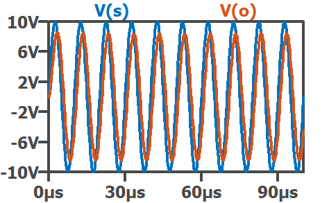
Waveforms of the simple R-C circuit simulation
Using LTSpice params
In LTspice parameters are variables that can be reused throughout the schematic. They are defined with the .op SPICE directive ".param <name> = <value>". For example, we can parameterize the capacitance C1 in this simulation with the following modifications to the schematic.
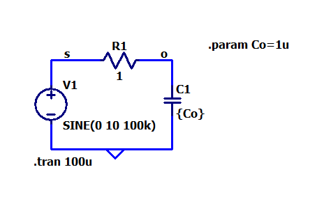
parameterized capacitance in the R-C circuit
Waveforms of the parameterized R-C circuit simulation
Note that the capacitance value is now {Co}. Co is the name of the parameter we have defined, and the curly braces let LTspice know that there is an expression that needs to be evaluated before executing the simulation. Also note that the waveforms are completely unchanged -- since we have parameterized the capacitance, but still given it a value of 1 uF, the circuit being simulated is unchanged.
To get some use out of the parameter, we now look at sweeping the value over a range. This can be accomplished with the .op SPICE directive ".step". The step command operates similar to a for-loop in spice. We can use the step command to change sources, temperature, or parameters. We'll focus on the latter. A couple options for syntax for this .op command are
-
.step param <name> <start> <stop> <step>Steps parameter <name> from <start> to <stop> in steps of size <step> -
.step param <name> list <val1> <val2> <val3> ...Steps parameter <name> over a list of specified values, <val1> <val2> <val3> ...
Using the former, we get the following. Each individual waveform is one capacitance value between 1 uF and 10 uF, with steps of 1uF
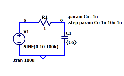
stepped parameter in R-C circuit simulation
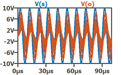
Waveforms of R-C circuit simulation with stepped output capacitance
Often, we care predominately about some specific characteristic of the waveforms. For example, if we want to only know the average value of the output voltage, we can direct LTspice to measure it with the .meas directive, as in the following.
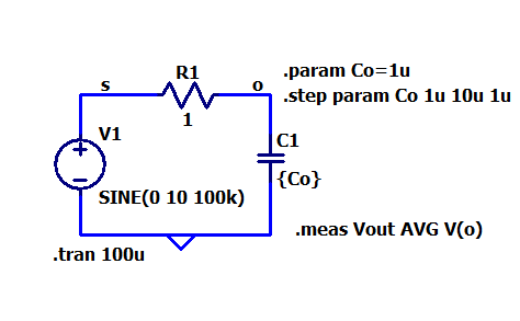
Adding a .meas command to the circuit
In this case, LTspice will measure and record the average (AVG) value of signal V(o) and save it into a variable named Vout. These measurements aren't directly available for plotting, however. Instead, we need to find them in the SPICE log, under View >> SPICE Error Log. In the error log, you will find a table of measurements, which can be right-clicked and plotted as shown below.
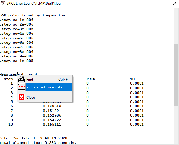
SPICE Error Log: measured data
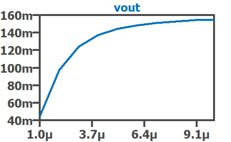
plotted .step'ed .meas data
Alternately, without using .meas, it is possible to change the x-axis of the simulation plot to a parameter value. For example, by right-clicking on the x-axis of the transient result plot, the "time" axis can be changed to Co. Since time-domain waveforms are still being plotted, we see the range of the sinusoid at V(o) in the plot above each capacitance value.
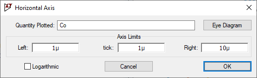
x-axis right-click menu
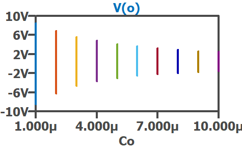
Vout(t) versus capacitance value
Of course, we can also plot formulas in this window. As an example, by right-clicking on the trace name, the following plots the instantaneous power dissipated on resistor R1 for each capacitance value
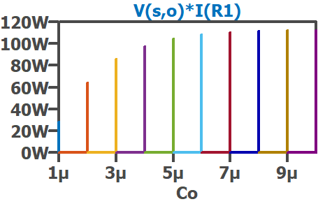
instantaneous power dissipation on the resistor, for varying capacitance
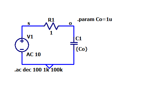
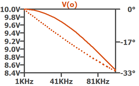
Often, this approach is less useful in a time-domain simulation due to the presence of time-varying signals. However, if we convert to an ac simulation (i.e. phasor-domain), we can use this more widely. In the following, the source has been changed from a sinusoidal time-domain voltage source, to an ac source with amplitude 10. The simulation command has been changed from .tran to .ac, an ac simulation with just a single frequency of 100kHz. Running the simulation, Spice automatically plots with the x-axis equal to the swept parameter (if simulation is only for a single frequency). The plots now show the magnitude and phase of the selected signals.
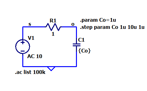
ac simulation with stepped parameter
ac simulation plot of V(o) for varying capacitance
Note that the magnitude will be displayed in dB scale by default. This can be changed to linear scale by right-clicking the (left) y-axis.
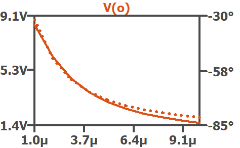
Alternately, we could instead sweep frequency. In this case, the simulation command is altered to sweep the source frequency from 1kHz to 100kHz, with 100 points per decade, spaced logarithmically.
ac simulation with stepped frequency
ac simulation plot of V(o) for varying frequency
Note: be careful about assessing power with this approach. Because we are working with phasors, we must use phasor calculations for power. As an example, the power dissipated in R1 for the above simulation is
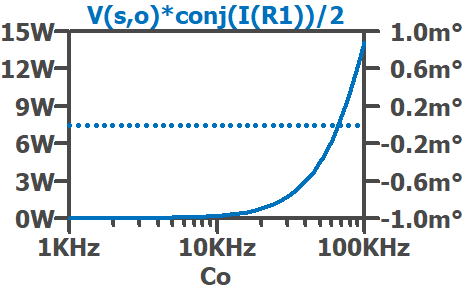
Phasor calculation for power dissipated in R1