ECE 692: Discrete Time Modeling of Power Electronics

Using PLECS to generate State Space Descriptions
In this class, we will use PLECS primarily to generate numerical state space descriptions from a graphical circuit model. The software has significant additional functionality which will not be covered in detail.
Installation
PLECS student licenses are available for UTK students in this class. A license can be obtained by e-mailing ithelp@eecs.utk.edu and requesting a student license. The EECS Department IT will guide you through the process thereafter. The licenses are available for students to install on personal (i.e. not UTK-owned) computers.
PLECS comes in both a Standalone and Blockset package. For the purposes of ECE692, we will be using the Blockset Package, which integrates with MATLAB/Simulink. The installer for PLECS Blockset is available at the following location.
It is best if you request and receive your license from EECS IT before installing, as the installer will ask you to provide the license during the installation process. If not, you can change/update the license at any time from the prompt that appears when starting PLECS.
To integrate with MATLAB, the m-files of the PLECS Blockset need to be visible in MATLAB. The installer will attempt to configure this for you, but occasionally does not succeed. If you are having trouble using PLECS in MATLAB, make sure that the PLECS directory is in the MATLAB path. You can do this programmatically in a single script through use of the addpath() function, or can permanently add the PLECS functions to the MATLAB default through the GUI by going to "Set Path" within the "Home" toolbar, and adding the PLECS Blockset installation directory to the path. On my machine, this appears as shown below.
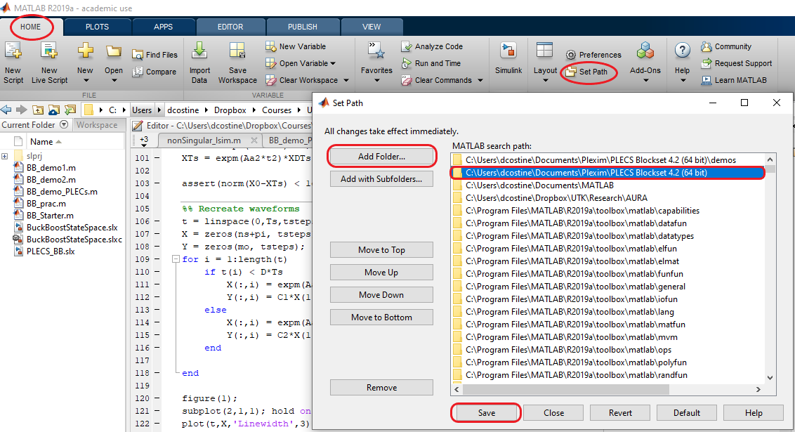
Editing the MATLAB path
Once installed and added to the MATLAB path, you should be able to type help plecs into the command line, and see a brief overview of available functions from PLECS, as shown below.
-
>> help plecsPLECSEDIT Command Line Interface for plecs. PLECSEDIT('CMD','PARAMETER1','PARAMETER2',...) allows you to access plecs component and circuit parameters directly from the MATLAB command line. 'CMD' is one of the following commands: get, set, hostid. PLECSEDIT('get','COMPONENT_PATH',['PARAMETER']) returns the value of PARAMETER of the plecs component indicated by the COMPONENT_PATH as a string. If PARAMETER is omitted a cell aray with all available parameters is returned. PLECSEDIT('set','COMPONENT_PATH', 'PARAMETER', 'VALUE') set the value of PARAMETER of the plecs component indicated by the COMPONENT_PATH to 'VALUE'. PLECSEDIT('hostid') prints the hostid information. Examples: plecs('get', 'mdl/Circuit1') % returns the parameters of Circuit1 % in the simulink model mdl plecs('get', 'mdl/Circuit1', 'Name') % returns the name of Circuit1 plecs('get', 'mdl/Circuit1', 'CircuitModel') % returns the circuit simulation % method of Circuit1 plecs('get', 'mdl/Circuit1/R1') % returns the parameters of component % R1 in circuit Circuit1 plecs('set', 'mdl/Circuit1/R1', 'R', '2') % sets the resistance of component % R1 in circuit Circuit1 to 2
PLECS Blockset: State Space Model Extraction
For the purposes of this tutorial, the main useage of PLECS is to generate a state space model of a circuit diagram. To do so, create a new Simulink model and add a PLECS Circuit from the library browser. Double-click the PLECS Circuit to open the PLECS circuit editor, and sketch your circuit. Use only electrical passives, sources, meters, and generic MOSFET elements. In the following, the MOSFETs will become ideal switches, all inductor currents and capacitor voltages will become states $x$, sources will become inputs $u$, and meters will become outputs $y$ in the state space model. Example screenshots for the creation of the buck-boost from lecture are shown below.

Adding a PLECS circuit from the Simulink Library
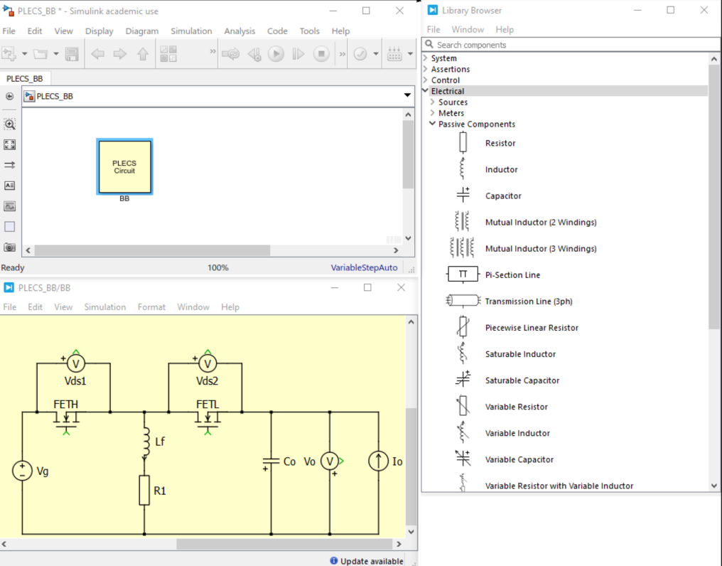
Simulink model, PLECS circuit, and PLECS library browser
To extract the state space model, you do not need to connect the MOSFET gates, or meter outputs
Once your model is created, return to MATLAB. There are three different PLECS commands which will be useful; their structure and output are shown below. In all three, 'mdl/circuit' is the path to the PLECS circuit you are analyzing, through the Simulink model that it is embedded in. For example, in the above figures, 'mdl/circuit' would be 'PLECS_BB/BB', where PLECS_BB is the name of the Simulink .mdl file and BB is the name of the PLECS circuit contained within it.
When all three commands are used, the result is a state-space description of the PLECS circuit which can be used in calculations in MATLAB
-
>> vec = plecs('get', 'mdl/circuit', 'StateSpaceOrder')vec = struct with fields: States: {ns×1 cell} Inputs: {pi×1 cell} Outputs: {mo×1 cell} Switches: {nsw×1 cell}This command returns the structure of the state, input, output, and switch vectors. PLECS creates these vectors as you edit the schematic, so the ordering of elements within each vector depends on the order that you added the elements to the schematic.
vec.Stateswill contain the names of all $n_s$ capacitors and inductors,vec.Inputscontains all $p_i$ sources,vec.Outputscontains all $m_o$ meters, andvec.Switchescontains all $n_{sw}$ semiconductor switches.It is important to examine these vectors, as PLECS may not natively arrange the elements in these vectors in the order that you expect. The order can be altered by removing and re-inserting any element, which will move it to the end of the vector. Make sure that the content and arrangement of each vector matches your expectations.
-
>> plecs('set', 'mdl/circuit', 'SwitchVector', swVec)This command produces no output, but sets the on-off state of each of the switches (MOSFET symbols) in the circuit. For example, setting
swVec=[0 1]will replace the first element in theSwitchesvector with its on-state model, and the second element with its off-state model. For MOSFETs, this means the first switch is replaced with a resistance $r_{on}$ and the second switch is left open. -
>> model = plecs('get', 'mdl/circuit', 'Topology')ans = struct with fields: A: [ns×ns double] B: [ns×pi double] C: [mo×ns double] D: [mo×pi double] I: [ns×ns double]This command returns the state-space description of the circuit, with the specified switch configuration from the previous command.
$$\dot{\bf x}(t) = {\bf A}{\bf x}(t) + {\bf B}{\bf u}(t) $$ $${\bf y}(t) = {\bf C}{\bf x}(t) + {\bf D}{\bf u}(t) $$model.A,model.B,model.C, andmodel.Dare numerical matrices which conform to the state space description of the system,Iis discussed further in the Model Order Reduction section, below
Additional Notes
-
State Order Reduction
model.Iis an additional matrix which contains information about model-order reductions in the system. Ifmodel.Icontains an identity matrix, no model order reduction has taken place.If
model.Iis not exactly the identity matrix, then there was at least one capacitive loop or inductive cutset in the circuit. When deriving by hand, this means that the number of states of the circuit is less than the number of reactive components. In this case, PLECS keeps all reactive elements in the state space model, but identifies which states were not actually used in the model for a complete description of the circuit throughmodel.I. Those states that are not used are denoted by the rows ofmodel.Iwhich do not match the identity matrix of the same size.The idea is that
model.Iwill "act" as an identity matrix for the state vector. So, if we multiple $x(t)$ bymodel.I, we should get back $x(t)$. For the rows ofmodel.Iwhich match the identity matrix, this is straighforward. For those which don't, the row inmodel.Iwill show how that state can be derived solely from other states of the system. For example, ifmodel.I = 0 0 1 1 1 0 1 0 0 0 0 0 1 0 0 0 0 0 1 0 0 0 0 0 1The second through fifth elements of
vec.Statesare the actual states of the model, and the first element can be reproduced through the sum of the last three entries ofvec.States. In this case, you should see that the first column ofmodel.Ais also equal to zero, indicating that no states depend in any way on the value of the first state invec.States.In some cases, it will be better to remove these state(s) from the circuit model, by deleting the corresponding rows and columns from the state space matrices. The signal can always be recovered later from the relationship shown by its corresponding row in
model.I -
Parameterized Models
With every call to
plecs('get', 'mdl/circuit', 'Topology'), PLECS will replace any variables in the model with their associated value in the workspace. In this was, the inductance of an inductor can be set toLin the circuit model, then if the calling MATLAB script first definesL=1e-6, the resulting state space matrices will be evaluated with a one microHenry inductance. The same holds of other parameters of circuit model elements (passive values, sources, MOSFET resistances, etc.)Note that changing
Lin the MATLAB script after the call to plecs will not change the state space model unlessplecs('get', 'mdl/circuit', 'Topology')is re-run -
State Space Splitting
PLECS has a feature called "State-Space Splitting" which is turned on by default for new models. This feature is used when PLECS notices that the model can be divided into multiple, smaller state space descriptions with dynamics which are well separated in the frequency domain. This is useful in time-stepping simulations, as when fast dynamics occur, only a subset of the model needs to be evaluated with small time-steps, while the remainder can be evaluated at a slower rate, reducing simulation time.
However, for our purposed, this option will result in an incomplete state space description being returned when MATLAB calls PLECS. As such, it is best to turn this off when using PLECS for a circuit state space parser. This can be done within a PLECS circuit by going to Simluation → PLECS Parameters → Advanced (tab) and unchecking "Enable state-space splitting".
-
State-Source Dependence
PLECS throws an error when any loop contains one or more voltage sources and otherwise all capacitors, or any cutset contains one or more current sources and otherwise all inductors. In this case, an attempt to parse the state space from PLECS will throw a "state-source dependence" error.
In most cases for our work, this configuration is not problematic because we consider only DC sources. However, for a time varying source, either configuration will result in some dependence of the states on the time-derivative of the source. For example, a capacitor $C$ in parallel with a time varying voltage source $v(t)$ will have current $$i_c(t) = \frac{d}{dt}v(t)$$ Therefore $$\frac{d}{dt}v_c(t) = \frac{1}{C}\frac{d}{dt}v(t)$$ which indicates a state space description of the form $$\dot{\bf x}(t) = {\bf A}{\bf x}(t) + {\bf B}{\bf u}(t) + {\bf \beta}\dot{\bf u}(t) $$ is necessary. This form of state space description is commonly used in certain applications, but is not necessary for the purposes of this course. Instead, the error in PLECS can be remedied by adding a small series resistance or parallel conductance to the voltage or current source(s), respectively.