Next: Application to Reduced-Order Modeling
Up: Band Lanczos Method
Previous: Basic Properties
Contents
Index
A complete statement of the band Lanczos algorithm is as follows.
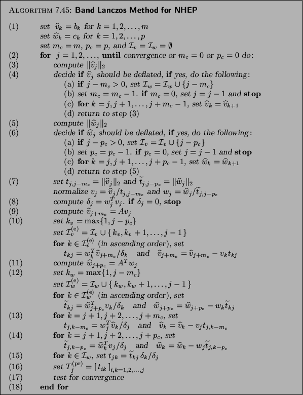
We stress that the non-Hermitian band Lanczos method can
be implemented by directly following the statement
in Algorithm 7.16, together with the further
details of some of the steps given below.
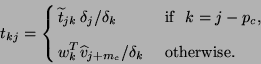
To keep the length of the statement
to one page, in Algorithm 7.16, all potentially
nonzero entries of the banded parts of  and
and  are computed as inner products.
However, only roughly half of these entries need to be explicitly
computed as inner products.
The remaining entries
can be obtained via the relation
 |
(185) |
which follows from the connection (7.71) of
 and
and
 .
In particular, in the following discussion of steps (10), (12), (13),
and (14), we give formulas for the entries of and
that use (7.79) whenever possible.
Employing these formulas would minimize the number of inner
products, but it would sacrifice some numerical stability.
.
In particular, in the following discussion of steps (10), (12), (13),
and (14), we give formulas for the entries of and
that use (7.79) whenever possible.
Employing these formulas would minimize the number of inner
products, but it would sacrifice some numerical stability.
Next, we discuss some of the steps of Algorithm 7.16
in more detail.
- (4)
- Generally, the decision if
 needs to be deflated should
be based on checking if
needs to be deflated should
be based on checking if
 |
(186) |
where  is a suitably chosen small deflation tolerance.
The vector is then deflated if (7.80) is
satisfied.
In this case, the value
is a suitably chosen small deflation tolerance.
The vector is then deflated if (7.80) is
satisfied.
In this case, the value  , if positive, is added to the index
set
, if positive, is added to the index
set  , which contains the indices of the nonzero rows
in the part
, which contains the indices of the nonzero rows
in the part
 of , and the current
right block size is updated to
of , and the current
right block size is updated to  .
If
.
If  , then the right block Krylov sequence (7.60) is
exhausted, and the algorithm terminates naturally.
If
, then the right block Krylov sequence (7.60) is
exhausted, and the algorithm terminates naturally.
If  , the vector
  is deleted, the index
  of each of the remaining right candidate vectors
  is
reset to
is
reset to  , and, finally, the algorithm returns to step (3).
If (7.80) is not satisfied, then no deflation is
necessary and the algorithm proceeds with step (5).
, and, finally, the algorithm returns to step (3).
If (7.80) is not satisfied, then no deflation is
necessary and the algorithm proceeds with step (5).
- (6)
- In analogy to (7.80),
the decision if
 needs to be deflated is based on checking
if
needs to be deflated is based on checking
if
 |
(187) |
The vector is then deflated if (7.81) is
satisfied.
In this case, the value  , if positive, is added to the index
set
, if positive, is added to the index
set  , which contains the indices of the nonzero rows
in the part
, which contains the indices of the nonzero rows
in the part
 of , and the current
left block size is updated to
of , and the current
left block size is updated to  .
If
.
If  , then the left block Krylov sequence (7.61) is
exhausted, and the algorithm terminates naturally.
If
, then the left block Krylov sequence (7.61) is
exhausted, and the algorithm terminates naturally.
If  , the vector is deleted, the index
of each of the remaining left candidate vectors
, the vector is deleted, the index
of each of the remaining left candidate vectors  is
reset to , and finally, the algorithm returns to step (5).
If (7.81) is not satisfied, then no deflation is
necessary and the algorithm proceeds with step (7).
is
reset to , and finally, the algorithm returns to step (5).
If (7.81) is not satisfied, then no deflation is
necessary and the algorithm proceeds with step (7).
- (7)
- Both vectors and have passed the deflation
check and are now normalized to become the next right and left
Lanczos vectors
 and
and  , respectively.
The normalization is such that
, respectively.
The normalization is such that
- (8)
- Here, we compute
 and check for breakdown.
If
and check for breakdown.
If  , then look-ahead would be needed in order
to continue the algorithm.
, then look-ahead would be needed in order
to continue the algorithm.
- (9)
- In this step, we advance the right block Krylov sequence by
computing a new candidate vector,
 , as the
 -multiple of the latest right Lanczos vector .
- (10)
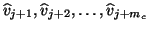
- The vector
is biorthogonalized against the left
Lanczos vectors
 ,
,
 .
Note that a TSMGS procedure is used to do
this biorthogonalization.
.
Note that a TSMGS procedure is used to do
this biorthogonalization.
One of the inner products required in the computation of  can be saved by employing (7.79).
More precisely, the following formula for should be used:
can be saved by employing (7.79).
More precisely, the following formula for should be used:
 |
(188) |
Note that the necessary entry
 in (7.82)
is available from step (7).
in (7.82)
is available from step (7).
- (11)
- In this step, we advance the left block Krylov sequence by
computing a new candidate vector,
 , as the
 -multiple of the latest left Lanczos vector .
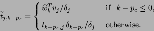
- (12)
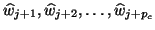
- The vector
is
biorthogonalized against the right Lanczos vectors
 ,
,
 .
Note that this biorthogonalization is done by means of
a TSMGS procedure.
Again, to save one inner product, the following formula for
.
Note that this biorthogonalization is done by means of
a TSMGS procedure.
Again, to save one inner product, the following formula for
 should be used:
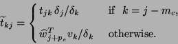
- (13)
- The right candidate vectors,
 , are
biorthogonalized against the latest left Lanczos vector .
To save inner products, the following formula for
, are
biorthogonalized against the latest left Lanczos vector .
To save inner products, the following formula for  could be used:
However, the use of this formula sacrifices some numerical stability.![[*]](http://www.netlib.org/utk/icons/footnote.png)
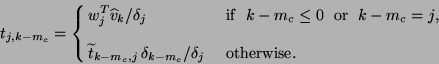
- (14)
- The left candidate vectors,
 , are
biorthogonalized against the latest right Lanczos
vector .
To save inner products, the following formula for
, are
biorthogonalized against the latest right Lanczos
vector .
To save inner products, the following formula for
 could be used:
However, the use of this formula sacrifices some numerical stability.
- (15)
- The entries
 computed in this step are the
potentially nonzero entries in the
computed in this step are the
potentially nonzero entries in the  th row of
 due to the vertical spikes caused by the deflation of
  vectors.
Note that again formula (7.79) is employed.
vectors.
Note that again formula (7.79) is employed.
- (16)
- All the potentially nonzero elements in the
th row and the th column of
have now been computed and they are added to the
matrix
 of the previous iteration
  , to yield
the current matrix
, to yield
the current matrix
 .
Here, we use the convention that entries
.
Here, we use the convention that entries  that are not explicitly defined in Algorithm 7.16 are set
to be zero.
We remark that in the initial iterations, i.e., as long as
that are not explicitly defined in Algorithm 7.16 are set
to be zero.
We remark that in the initial iterations, i.e., as long as
 , respectively
  , Algorithm 7.16
also produces entries , respectively
,
with negative indices
, Algorithm 7.16
also produces entries , respectively
,
with negative indices  .
These entries arise from the biorthogonalization of the
starting vectors, and they are not part of the matrix
.
In particular, these entries are not needed when
Algorithm 7.16 is used for eigenvalue computations.
However, they are crucial when Algorithm 7.16
is applied to reduced-order modeling, as we will discuss
in §7.10.4 below.
.
These entries arise from the biorthogonalization of the
starting vectors, and they are not part of the matrix
.
In particular, these entries are not needed when
Algorithm 7.16 is used for eigenvalue computations.
However, they are crucial when Algorithm 7.16
is applied to reduced-order modeling, as we will discuss
in §7.10.4 below.
- (17)
- For eigenvalue computations, one tests for convergence by
computing the eigenvalues
 ,
,
 , of
the
, of
the  matrix
.
The algorithm is stopped if some of the
's are
good enough approximations to the desired eigenvalues of .
For reduced-order modeling, the algorithm is stopped if
the th-order model generated by the algorithm is
a good enough approximation of the original linear dynamical
system.
matrix
.
The algorithm is stopped if some of the
's are
good enough approximations to the desired eigenvalues of .
For reduced-order modeling, the algorithm is stopped if
the th-order model generated by the algorithm is
a good enough approximation of the original linear dynamical
system.
Next: Application to Reduced-Order Modeling
Up: Band Lanczos Method
Previous: Basic Properties
Contents
Index
Susan Blackford
2000-11-20