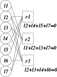
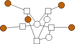
Figure 1. An example Tanner graph for n=4 and m=3.
Technical Report CS-03-528.
Department of Computer Science
University of Tennessee
203 Claxton Complex
Knoxville, TN 37996-3450
July, 2004.
See http://web.eecs.utk.edu/~jplank/plank/papers/CS-04-528.html for the publication status of this paper.
plank@cs.utk.edu
http://web.eecs.utk.edu/~jplank
Let the number of data bits be n, and the number of coding bits be m. Let the average number of bits required to decode all bits in the code be o, otherwise termed the "overhead". Finally, let the computational overhead of a code be l.
In this paper, we present the optimal systematic codes for each value of n, m and l, such that (n+m)*m is less than or equal to 30. These codes have been derived by an exhaustive search of all codes. It is the intent of this paper to provide systems researchers and programmers with a reference that they may use when they need to evaluate and employ small codes in their applications.
In this paper, we present optimally performing, small codes. Optimality is determined as follows. We are given three parameters:
For each value of n, m and l, we present codes that minimize the "overhead" o, defined to be the average number of bits required to reconstruct all the bits of the code.
Since the intent of this paper is to be a reference for systems programmers, its organization is a little eccentric. We first present the basics of coding, how bipartite graphs represent codes, and how to encode and decode given a bipartite graph. We then present optimal codes for all values of n and m such that (n+m)*n is less than or equal to 30. Following that, we present the exact mechanics of encoding, decoding, and computing overhead.
Parity-check codes are based on bipartite graphs known as "Tanner" graphs. These graphs have n+m nodes on their left side, sometimes termed the "message" nodes, and m nodes on their right side, termed "check" nodes. Edges only connect message and check nodes. An example graph is depicted in Figure 1.

Figure 1. An example Tanner graph for n=4 and m=3.
The left-hand nodes hold the bits that are to be stored by the application. The edges and the right-hand nodes specify constraints that the left-hand nodes must satisfy. The most straightforward codes are "systematic" codes, where the data bits are stored in n of the left-hand nodes, and the coding bits in the remaining m left-hand nodes are calculated from the data bits and the constraints in the right-hand nodes using exclusive-or.
For example the code in Figure 1, is a systematic one, whose data bits may be stored in nodes l1 through l4. The coding bits are calculated as follows:
We present decoding as an act in a storage system. Suppose we store each of the (n+m) bits on a different storage node. Then we download bits from the storage nodes at random until we have downloaded enough bits to reconstruct the data. To decode in this manner, we start with the Tanner graph for the code, placing values of zero in each right-hand node, and leaving the left-hand nodes empty. When we download a bit, we put its value into its corresponding left-hand hand node lx. Then, for each right-hand node rx to which it is connected, we update the value stored in rx to be the exclusive-or of that value and the value in lx. We then remove the edge (lx,rx), from the graph. At the end of this process, if there are any right-hand nodes with only one incident edge, then they contain the decoded values of the left-hand node to which they are connected, and we can set the value of those left-hand nodes accordingly, and then remove their edges from the graph in the same manner as if they had been downloaded. Obviously, this is an iterative process.
When all nodes' values have been either downloaded or decoded, the decoding process is finished. If a code is systematic, then the data bits are held in n of the left-hand nodes. The number of exclusive-or/copy operations required is equal to the number of edges in the graph.
Encoding with a systematic graph is straightforward -- simply decode using the n data bits.
The optimal overhead of any decoding scheme is n. Therefore, the overhead factor f(G) of a graph Gis o(G)/n, and the optimal overhead factor of any decoding scheme is 1. Note, Reed-Solomon coding achieves this optimimum; however, its large (O(n*n)) computational overhead renders it unattractive for many applications.
In [PT04], we used a Monte-Carlo simulation to estimate the overhead factor of various codes. In this paper, we determine overhead factor exactly, using a recursive formula. However, before presenting this determination, we describe the optimal codes.
The table that follows presents optimal codes in the following format. First, n, m, l, o(G), and f(G) are listed, then a list of the edges of each left-hand node in the graph, and then finally a list of the coding nodes of the graph. The nodes are zero-indexed. As an example, consider the following table entry:
| n | m | l | o(G) | f(G) | Edges of G | Coding Nodes |
| 3 | 3 | 9 and up | 3.2000 | 1.0667 | {(0)(1)(0,1)(2)(0,2)(1,2)} | {0,1,3} |
This says that for n=3 and m=3, and for all values of l greater than or equal to nine, the following graph is optimal, having an overhead of 3.2 and an overhead factor of 1.0667:
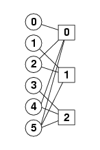
Moreover, the graph is systematic, with coding nodes 0, 1 and 3, and data nodes 2, 4 and 5. Note, the graph has 9 edges, as denoted by the l column.
Note, if all graphs for a value of l have overhead factors greater than a graph with a smaller value of l, then the latter graph will perform better in terms of both overhead factor and decoding performance. For that reason, as in the above table entry, if a graph for a certain value of l has a smaller overhead factor than all graphs with higher values of l, we list that graph as the optimal for that value of l "and up."
Tables 1, 2 and 3 list the optimal graphs for (n+m)*m <= 30 and m > 1. (We do not present graphs for m=1 as straight parity is optimal in these cases.)
| n | m | l | o(G) | f(G) | Edges of G | Coding Nodes |
| 2 | 2 | 4 | 2.3333 | 1.1667 | {(0)(0)(1)(1)} | 0,2 |
| 2 | 2 | 5 and up | 2.1667 | 1.0833 | {(0)(1)(1)(0,1)} | 0,1 |
| 3 | 2 | 5 | 3.4000 | 1.1333 | {(0)(0)(1)(1)(1)} | 0,2 |
| 3 | 2 | 6 and up | 3.2000 | 1.0667 | {(0)(0)(1)(1)(0,1)} | 0,2 | 4 | 2 | 6 | 4.4000 | 1.1000 | {(0)(0)(0)(1)(1)(1)} | 0,3 |
| 4 | 2 | 7 | 4.2667 | 1.0667 | {(0)(0)(1)(1)(1)(0,1)} | 0,2 |
| 4 | 2 | 8 and up | 4.2000 | 1.0500 | {(0)(0)(1)(1)(0,1)(0,1)} | 0,2 |
| 5 | 2 | 7 | 5.4286 | 1.0857 | {(0)(0)(0)(1)(1)(1)(1)} | 0,3 |
| 5 | 2 | 8 | 5.2857 | 1.0571 | {(0)(0)(0)(1)(1)(1)(0,1)} | 0,3 |
| 5 | 2 | 9 and up | 5.2381 | 1.0476 | {(0)(0)(1)(1)(1)(0,1)(0,1)} | 0,2 |
| 6 | 2 | 8 | 6.4286 | 1.0714 | {(0)(0)(0)(0)(1)(1)(1)(1)} | 0,4 |
| 6 | 2 | 9 | 6.3214 | 1.0536 | {(0)(0)(0)(1)(1)(1)(1)(0,1)} | 0,3 |
| 6 | 2 | 10 and up | 6.2500 | 1.0417 | {(0)(0)(0)(1)(1)(1)(0,1)(0,1)} | 0,3 |
| 7 | 2 | 9 | 7.4444 | 1.0635 | {(0)(0)(0)(0)(1)(1)(1)(1)(1)} | 0,4 |
| 7 | 2 | 10 | 7.3333 | 1.0476 | {(0)(0)(0)(0)(1)(1)(1)(1)(0,1)} | 0,4 |
| 7 | 2 | 11 | 7.2778 | 1.0397 | {(0)(0)(0)(1)(1)(1)(1)(0,1)(0,1)} | 0,3 |
| 7 | 2 | 12 and up | 7.2500 | 1.0357 | {(0)(0)(0)(1)(1)(1)(0,1)(0,1)(0,1)} | 0,3 |
| 8 | 2 | 10 | 8.4444 | 1.0556 | {(0)(0)(0)(0)(0)(1)(1)(1)(1)(1)} | 0,5 |
| 8 | 2 | 11 | 8.3556 | 1.0444 | {(0)(0)(0)(0)(1)(1)(1)(1)(1)(0,1)} | 0,4 |
| 8 | 2 | 12 | 8.2889 | 1.0361 | {(0)(0)(0)(0)(1)(1)(1)(1)(0,1)(0,1)} | 0,4 |
| 8 | 2 | 13 and up | 8.2667 | 1.0333 | {(0)(0)(0)(1)(1)(1)(1)(0,1)(0,1)(0,1)} | 0,3 |
| 9 | 2 | 11 | 9.4545 | 1.0505 | {(0)(0)(0)(0)(0)(1)(1)(1)(1)(1)(1)} | 0,5 |
| 9 | 2 | 12 | 9.3636 | 1.0404 | {(0)(0)(0)(0)(0)(1)(1)(1)(1)(1)(0,1)} | 0,5 |
| 9 | 2 | 13 | 9.3091 | 1.0343 | {(0)(0)(0)(0)(1)(1)(1)(1)(1)(0,1)(0,1)} | 0,4 |
| 9 | 2 | 14 and up | 9.2727 | 1.0303 | {(0)(0)(0)(0)(1)(1)(1)(1)(0,1)(0,1)(0,1)} | 0,4 |
| 10 | 2 | 12 | 10.4545 | 1.0455 | {(0)(0)(0)(0)(0)(0)(1)(1)(1)(1)(1)(1)} | 0,6 |
| 10 | 2 | 13 | 10.3788 | 1.0379 | {(0)(0)(0)(0)(0)(1)(1)(1)(1)(1)(1)(0,1)} | 0,5 |
| 10 | 2 | 14 | 10.3182 | 1.0318 | {(0)(0)(0)(0)(0)(1)(1)(1)(1)(1)(0,1)(0,1)} | 0,5 |
| 10 | 2 | 15 | 10.2879 | 1.0288 | {(0)(0)(0)(0)(1)(1)(1)(1)(1)(0,1)(0,1)(0,1)} | 0,4 |
| 10 | 2 | 16 and up | 10.2727 | 1.0273 | {(0)(0)(0)(0)(1)(1)(1)(1)(0,1)(0,1)(0,1)(0,1)} | 0,4 |
| 11 | 2 | 13 | 11.4615 | 1.0420 | {(0)(0)(0)(0)(0)(0)(1)(1)(1)(1)(1)(1)(1)} | 0,6 |
| 11 | 2 | 14 | 11.3846 | 1.0350 | {(0)(0)(0)(0)(0)(0)(1)(1)(1)(1)(1)(1)(0,1)} | 0,6 |
| 11 | 2 | 15 | 11.3333 | 1.0303 | {(0)(0)(0)(0)(0)(1)(1)(1)(1)(1)(1)(0,1)(0,1)} | 0,5 |
| 11 | 2 | 16 | 11.2949 | 1.0268 | {(0)(0)(0)(0)(0)(1)(1)(1)(1)(1)(0,1)(0,1)(0,1)} | 0,5 |
| 11 | 2 | 17 and up | 11.2821 | 1.0256 | {(0)(0)(0)(0)(1)(1)(1)(1)(1)(0,1)(0,1)(0,1)(0,1)} | 0,4 |
| 12 | 2 | 14 | 12.4615 | 1.0385 | {(0)(0)(0)(0)(0)(0)(0)(1)(1)(1)(1)(1)(1)(1)} | 0,7 |
| 12 | 2 | 15 | 12.3956 | 1.0330 | {(0)(0)(0)(0)(0)(0)(1)(1)(1)(1)(1)(1)(1)(0,1)} | 0,6 |
| 12 | 2 | 16 | 12.3407 | 1.0284 | {(0)(0)(0)(0)(0)(0)(1)(1)(1)(1)(1)(1)(0,1)(0,1)} | 0,6 |
| 12 | 2 | 17 | 12.3077 | 1.0256 | {(0)(0)(0)(0)(0)(1)(1)(1)(1)(1)(1)(0,1)(0,1)(0,1)} | 0,5 |
| 12 | 2 | 18 and up | 12.2857 | 1.0238 | {(0)(0)(0)(0)(0)(1)(1)(1)(1)(1)(0,1)(0,1)(0,1)(0,1)} | 0,5 |
| 13 | 2 | 15 | 13.4667 | 1.0359 | {(0)(0)(0)(0)(0)(0)(0)(1)(1)(1)(1)(1)(1)(1)(1)} | 0,7 |
| 13 | 2 | 16 | 13.4000 | 1.0308 | {(0)(0)(0)(0)(0)(0)(0)(1)(1)(1)(1)(1)(1)(1)(0,1)} | 0,7 |
| 13 | 2 | 17 | 13.3524 | 1.0271 | {(0)(0)(0)(0)(0)(0)(1)(1)(1)(1)(1)(1)(1)(0,1)(0,1)} | 0,6 |
| 13 | 2 | 18 | 13.3143 | 1.0242 | {(0)(0)(0)(0)(0)(0)(1)(1)(1)(1)(1)(1)(0,1)(0,1)(0,1)} | 0,6 |
| 13 | 2 | 19 | 13.2952 | 1.0227 | {(0)(0)(0)(0)(0)(1)(1)(1)(1)(1)(1)(0,1)(0,1)(0,1)(0,1)} | 0,5 |
| 13 | 2 | 20 and up | 13.2857 | 1.0220 | {(0)(0)(0)(0)(0)(1)(1)(1)(1)(1)(0,1)(0,1)(0,1)(0,1)(0,1)} | 0,5 |
| 2 | 3 | 6 | 2.5000 | 1.2500 | {(0)(0)(1)(2)(1,2)} | 0,2,3 |
| 2 | 3 | 7 and up | 2.2000 | 1.1000 | {(0)(1)(2)(0,2)(1,2)} | 0,1,2 |
| 3 | 3 | 6 | 3.8000 | 1.2667 | {(0)(0)(1)(1)(2)(2)} | 0,2,4 |
| 3 | 3 | 7 | 3.6333 | 1.2111 | {(0)(0)(1)(2)(2)(1,2)} | 0,2,3 |
| 3 | 3 | 8 | 3.4167 | 1.1389 | {(0)(1)(1)(2)(0,2)(1,2)} | 0,1,3 |
| 3 | 3 | 9 and up | 3.2000 | 1.0667 | {(0)(1)(0,1)(2)(0,2)(1,2)} | 0,1,3 |
| 4 | 3 | 7 | 4.8952 | 1.2238 | {(0)(0)(1)(1)(2)(2)(2)} | 0,2,4 |
| 4 | 3 | 8 | 4.6857 | 1.1714 | {(0)(0)(1)(1)(2)(2)(1,2)} | 0,2,4 |
| 4 | 3 | 9 | 4.4952 | 1.1238 | {(0)(0)(1)(1)(2)(0,2)(1,2)} | 0,2,4 |
| 4 | 3 | 10 | 4.3619 | 1.0905 | {(0)(1)(0,1)(2)(2)(0,2)(1,2)} | 0,1,3 |
| 4 | 3 | 12 and up | 4.2857 | 1.0714 | {(0)(1)(0,1)(2)(0,2)(1,2)(0,1,2)} | 0,1,3 |
| 5 | 3 | 8 | 5.9286 | 1.1857 | {(0)(0)(1)(1)(1)(2)(2)(2)} | 0,2,5 |
| 5 | 3 | 9 | 5.7500 | 1.1500 | {(0)(0)(0)(1)(1)(2)(2)(1,2)} | 0,3,5 |
| 5 | 3 | 10 | 5.5714 | 1.1143 | {(0)(0)(1)(1)(2)(2)(0,2)(1,2)} | 0,2,4 |
| 5 | 3 | 11 | 5.4464 | 1.0893 | {(0)(1)(1)(0,1)(2)(2)(0,2)(1,2)} | 0,1,4 |
| 5 | 3 | 12 | 5.4286 | 1.0857 | {(0)(0)(1)(0,1)(2)(0,2)(1,2)(1,2)} | 0,2,4 |
| 5 | 3 | 13 and up | 5.3750 | 1.0750 | {(0)(1)(0,1)(2)(2)(0,2)(1,2)(0,1,2)} | 0,1,3 |
| 6 | 3 | 9 | 6.9286 | 1.1548 | {(0)(0)(0)(1)(1)(1)(2)(2)(2)} | 0,3,6 |
| 6 | 3 | 10 | 6.8016 | 1.1336 | {(0)(0)(0)(1)(1)(2)(2)(2)(1,2)} | 0,3,5 |
| 6 | 3 | 11 | 6.6508 | 1.1085 | {(0)(0)(1)(1)(1)(2)(2)(0,2)(1,2)} | 0,2,5 |
| 6 | 3 | 12 | 6.4881 | 1.0813 | {(0)(0)(1)(1)(0,1)(2)(2)(0,2)(1,2)} | 0,2,5 |
| 6 | 3 | 13 | 6.4762 | 1.0794 | {(0)(0)(1)(0,1)(2)(2)(0,2)(1,2)(1,2)} | 0,2,4 |
| 6 | 3 | 14 and up | 6.4246 | 1.0708 | {(0)(1)(1)(0,1)(2)(2)(0,2)(1,2)(0,1,2)} | 0,1,4 |
| 7 | 3 | 10 | 7.9667 | 1.1381 | {(0)(0)(0)(1)(1)(1)(2)(2)(2)(2)} | 0,3,6 |
| 7 | 3 | 11 | 7.8250 | 1.1179 | {(0)(0)(0)(1)(1)(1)(2)(2)(2)(1,2)} | 0,3,6 |
| 7 | 3 | 12 | 7.6889 | 1.0984 | {(0)(0)(0)(1)(1)(1)(2)(2)(0,2)(1,2)} | 0,3,6 |
| 7 | 3 | 13 | 7.5694 | 1.0813 | {(0)(0)(1)(1)(0,1)(2)(2)(2)(0,2)(1,2)} | 0,2,5 |
| 7 | 3 | 14 | 7.5056 | 1.0722 | {(0)(0)(1)(1)(0,1)(2)(2)(0,2)(1,2)(1,2)} | 0,2,5 |
| 7 | 3 | 15 and up | 7.4500 | 1.0643 | {(0)(0)(1)(1)(0,1)(2)(2)(0,2)(1,2)(0,1,2)} | 0,2,5 |
| 8 | 3 | 11 | 8.9818 | 1.1227 | {(0)(0)(0)(1)(1)(1)(1)(2)(2)(2)(2)} | 0,3,7 |
| 8 | 3 | 12 | 8.8545 | 1.1068 | {(0)(0)(0)(0)(1)(1)(1)(2)(2)(2)(1,2)} | 0,4,7 |
| 8 | 3 | 13 | 8.7273 | 1.0909 | {(0)(0)(0)(1)(1)(1)(2)(2)(2)(0,2)(1,2)} | 0,3,6 |
| 8 | 3 | 14 | 8.6182 | 1.0773 | {(0)(0)(1)(1)(1)(0,1)(2)(2)(2)(0,2)(1,2)} | 0,2,6 |
| 8 | 3 | 15 | 8.5576 | 1.0697 | {(0)(0)(0)(1)(1)(0,1)(2)(2)(0,2)(1,2)(1,2)} | 0,3,6 |
| 8 | 3 | 16 | 8.5091 | 1.0636 | {(0)(0)(1)(1)(0,1)(2)(2)(0,2)(0,2)(1,2)(1,2)} | 0,2,5 |
| 8 | 3 | 17 and up | 8.4788 | 1.0598 | {(0)(0)(1)(1)(0,1)(2)(2)(0,2)(1,2)(1,2)(0,1,2)} | 0,2,5 |
| 9 | 3 | 12 | 9.9818 | 1.1091 | {(0)(0)(0)(0)(1)(1)(1)(1)(2)(2)(2)(2)} | 0,4,8 |
| 9 | 3 | 13 | 9.8818 | 1.0980 | {(0)(0)(0)(0)(1)(1)(1)(2)(2)(2)(2)(1,2)} | 0,4,7 |
| 9 | 3 | 14 | 9.7682 | 1.0854 | {(0)(0)(0)(1)(1)(1)(1)(2)(2)(2)(0,2)(1,2)} | 0,3,7 |
| 9 | 3 | 15 | 9.6455 | 1.0717 | {(0)(0)(0)(1)(1)(1)(0,1)(2)(2)(2)(0,2)(1,2)} | 0,3,7 |
| 9 | 3 | 16 | 9.5985 | 1.0665 | {(0)(0)(0)(1)(1)(0,1)(2)(2)(2)(0,2)(1,2)(1,2)} | 0,3,6 |
| 9 | 3 | 17 | 9.5515 | 1.0613 | {(0)(0)(1)(1)(1)(0,1)(2)(2)(0,2)(0,2)(1,2)(1,2)} | 0,2,6 |
| 9 | 3 | 18 | 9.5091 | 1.0566 | {(0)(0)(1)(1)(0,1)(0,1)(2)(2)(0,2)(0,2)(1,2)(1,2)} | 0,2,6 |
| 9 | 3 | 19 and up | 9.4939 | 1.0549 | {(0)(0)(1)(1)(0,1)(2)(2)(0,2)(0,2)(1,2)(1,2)(0,1,2)} | 0,2,5 |
| 10 | 3 | 13 | 11.0023 | 1.1002 | {(0)(0)(0)(0)(1)(1)(1)(1)(2)(2)(2)(2)(2)} | 0,4,8 |
| 10 | 3 | 14 | 10.8951 | 1.0895 | {(0)(0)(0)(0)(1)(1)(1)(1)(2)(2)(2)(2)(1,2)} | 0,4,8 |
| 10 | 3 | 15 | 10.7902 | 1.0790 | {(0)(0)(0)(0)(1)(1)(1)(1)(2)(2)(2)(0,2)(1,2)} | 0,4,8 |
| 10 | 3 | 16 | 10.6923 | 1.0692 | {(0)(0)(0)(1)(1)(1)(0,1)(2)(2)(2)(2)(0,2)(1,2)} | 0,3,7 |
| 10 | 3 | 17 | 10.6247 | 1.0625 | {(0)(0)(0)(1)(1)(1)(0,1)(2)(2)(2)(0,2)(1,2)(1,2)} | 0,3,7 |
| 10 | 3 | 18 | 10.5769 | 1.0577 | {(0)(0)(0)(1)(1)(1)(0,1)(2)(2)(0,2)(0,2)(1,2)(1,2)} | 0,3,7 |
| 10 | 3 | 19 | 10.5431 | 1.0543 | {(0)(0)(1)(1)(0,1)(0,1)(2)(2)(2)(0,2)(0,2)(1,2)(1,2)} | 0,2,6 |
| 10 | 3 | 20 | 10.5268 | 1.0527 | {(0)(0)(1)(1)(1)(0,1)(2)(2)(0,2)(0,2)(1,2)(1,2)(0,1,2)} | 0,2,6 |
| 10 | 3 | 21 and up | 10.5035 | 1.0503 | {(0)(0)(1)(1)(0,1)(0,1)(2)(2)(0,2)(0,2)(1,2)(1,2)(0,1,2)} | 0,2,6 |
| 11 | 3 | 14 | 12.0110 | 1.0919 | {(0)(0)(0)(0)(1)(1)(1)(1)(1)(2)(2)(2)(2)(2)} | 0,4,9 |
| 11 | 3 | 15 | 11.9121 | 1.0829 | {(0)(0)(0)(0)(0)(1)(1)(1)(1)(2)(2)(2)(2)(1,2)} | 0,5,9 |
| 11 | 3 | 16 | 11.8132 | 1.0739 | {(0)(0)(0)(0)(1)(1)(1)(1)(2)(2)(2)(2)(0,2)(1,2)} | 0,4,8 |
| 11 | 3 | 17 | 11.7225 | 1.0657 | {(0)(0)(0)(1)(1)(1)(1)(0,1)(2)(2)(2)(2)(0,2)(1,2)} | 0,3,8 |
| 11 | 3 | 18 | 11.6593 | 1.0599 | {(0)(0)(0)(0)(1)(1)(1)(0,1)(2)(2)(2)(0,2)(1,2)(1,2)} | 0,4,8 |
| 11 | 3 | 19 | 11.6016 | 1.0547 | {(0)(0)(0)(1)(1)(1)(0,1)(2)(2)(2)(0,2)(0,2)(1,2)(1,2)} | 0,3,7 |
| 11 | 3 | 20 | 11.5659 | 1.0514 | {(0)(0)(1)(1)(1)(0,1)(0,1)(2)(2)(2)(0,2)(0,2)(1,2)(1,2)} | 0,2,7 |
| 11 | 3 | 21 | 11.5467 | 1.0497 | {(0)(0)(0)(1)(1)(1)(0,1)(2)(2)(0,2)(0,2)(1,2)(1,2)(0,1,2)} | 0,3,7 |
| 11 | 3 | 22 and up | 11.5275 | 1.0480 | {(0)(0)(1)(1)(0,1)(0,1)(2)(2)(2)(0,2)(0,2)(1,2)(1,2)(0,1,2)} | 0,2,6 |
| 12 | 3 | 15 | 13.0110 | 1.0842 | {(0)(0)(0)(0)(0)(1)(1)(1)(1)(1)(2)(2)(2)(2)(2)} | 0,5,10 |
| 12 | 3 | 16 | 12.9289 | 1.0774 | {(0)(0)(0)(0)(0)(1)(1)(1)(1)(2)(2)(2)(2)(2)(1,2)} | 0,5,9 |
| 12 | 3 | 17 | 12.8381 | 1.0698 | {(0)(0)(0)(0)(1)(1)(1)(1)(1)(2)(2)(2)(2)(0,2)(1,2)} | 0,4,9 |
| 12 | 3 | 18 | 12.7407 | 1.0617 | {(0)(0)(0)(0)(1)(1)(1)(1)(0,1)(2)(2)(2)(2)(0,2)(1,2)} | 0,4,9 |
| 12 | 3 | 19 | 12.6886 | 1.0574 | {(0)(0)(0)(0)(1)(1)(1)(0,1)(2)(2)(2)(2)(0,2)(1,2)(1,2)} | 0,4,8 |
| 12 | 3 | 20 | 12.6344 | 1.0529 | {(0)(0)(0)(1)(1)(1)(1)(0,1)(2)(2)(2)(0,2)(0,2)(1,2)(1,2)} | 0,3,8 |
| 12 | 3 | 21 | 12.5802 | 1.0484 | {(0)(0)(0)(1)(1)(1)(0,1)(0,1)(2)(2)(2)(0,2)(0,2)(1,2)(1,2)} | 0,3,8 |
| 12 | 3 | 22 | 12.5641 | 1.0470 | {(0)(0)(0)(1)(1)(1)(0,1)(2)(2)(2)(0,2)(0,2)(1,2)(1,2)(0,1,2)} | 0,3,7 |
| 12 | 3 | 23 | 12.5436 | 1.0453 | {(0)(0)(1)(1)(1)(0,1)(0,1)(2)(2)(2)(0,2)(0,2)(1,2)(1,2)(0,1,2)} | 0,2,7 |
| 12 | 3 | 25 and up | 12.5407 | 1.0451 | {(0)(0)(1)(1)(0,1)(0,1)(2)(2)(2)(0,2)(0,2)(1,2)(1,2)(0,1,2)(0,1,2)} | 0,2,6 |
| 13 | 3 | 16 | 14.0238 | 1.0788 | {(0)(0)(0)(0)(0)(1)(1)(1)(1)(1)(2)(2)(2)(2)(2)(2)} | 0,5,10 |
| 13 | 3 | 17 | 13.9375 | 1.0721 | {(0)(0)(0)(0)(0)(1)(1)(1)(1)(1)(2)(2)(2)(2)(2)(1,2)} | 0,5,10 |
| 13 | 3 | 18 | 13.8524 | 1.0656 | {(0)(0)(0)(0)(0)(1)(1)(1)(1)(1)(2)(2)(2)(2)(0,2)(1,2)} | 0,5,10 |
| 13 | 3 | 19 | 13.7708 | 1.0593 | {(0)(0)(0)(0)(1)(1)(1)(1)(0,1)(2)(2)(2)(2)(2)(0,2)(1,2)} | 0,4,9 |
| 13 | 3 | 20 | 13.7083 | 1.0545 | {(0)(0)(0)(0)(1)(1)(1)(1)(0,1)(2)(2)(2)(2)(0,2)(1,2)(1,2)} | 0,4,9 |
| 13 | 3 | 21 | 13.6560 | 1.0505 | {(0)(0)(0)(0)(1)(1)(1)(1)(0,1)(2)(2)(2)(0,2)(0,2)(1,2)(1,2)} | 0,4,9 |
| 13 | 3 | 22 | 13.6107 | 1.0470 | {(0)(0)(0)(1)(1)(1)(0,1)(0,1)(2)(2)(2)(2)(0,2)(0,2)(1,2)(1,2)} | 0,3,8 |
| 13 | 3 | 23 | 13.5863 | 1.0451 | {(0)(0)(0)(1)(1)(1)(0,1)(0,1)(2)(2)(2)(0,2)(0,2)(1,2)(1,2)(1,2)} | 0,3,8 |
| 13 | 3 | 24 | 13.5536 | 1.0426 | {(0)(0)(0)(1)(1)(1)(0,1)(0,1)(2)(2)(2)(0,2)(0,2)(1,2)(1,2)(0,1,2)} | 0,3,8 |
| 13 | 3 | 26 and up | 13.5488 | 1.0422 | {(0)(0)(1)(1)(1)(0,1)(0,1)(2)(2)(2)(0,2)(0,2)(1,2)(1,2)(0,1,2)(0,1,2)} | 0,2,7 |
| 14 | 3 | 17 | 15.0294 | 1.0735 | {(0)(0)(0)(0)(0)(1)(1)(1)(1)(1)(1)(2)(2)(2)(2)(2)(2)} | 0,5,11 |
| 14 | 3 | 18 | 14.9485 | 1.0678 | {(0)(0)(0)(0)(0)(0)(1)(1)(1)(1)(1)(2)(2)(2)(2)(2)(1,2)} | 0,6,11 |
| 14 | 3 | 19 | 14.8676 | 1.0620 | {(0)(0)(0)(0)(0)(1)(1)(1)(1)(1)(2)(2)(2)(2)(2)(0,2)(1,2)} | 0,5,10 |
| 14 | 3 | 20 | 14.7912 | 1.0565 | {(0)(0)(0)(0)(1)(1)(1)(1)(1)(0,1)(2)(2)(2)(2)(2)(0,2)(1,2)} | 0,4,10 |
| 14 | 3 | 21 | 14.7324 | 1.0523 | {(0)(0)(0)(0)(0)(1)(1)(1)(1)(0,1)(2)(2)(2)(2)(0,2)(1,2)(1,2)} | 0,5,10 |
| 14 | 3 | 22 | 14.6765 | 1.0483 | {(0)(0)(0)(0)(1)(1)(1)(1)(0,1)(2)(2)(2)(2)(0,2)(0,2)(1,2)(1,2)} | 0,4,9 |
| 14 | 3 | 23 | 14.6324 | 1.0452 | {(0)(0)(0)(1)(1)(1)(1)(0,1)(0,1)(2)(2)(2)(2)(0,2)(0,2)(1,2)(1,2)} | 0,3,9 |
| 14 | 3 | 24 | 14.6074 | 1.0434 | {(0)(0)(0)(0)(1)(1)(1)(0,1)(0,1)(2)(2)(2)(0,2)(0,2)(1,2)(1,2)(1,2)} | 0,4,9 |
| 14 | 3 | 25 | 14.5794 | 1.0414 | {(0)(0)(0)(1)(1)(1)(0,1)(0,1)(2)(2)(2)(2)(0,2)(0,2)(1,2)(1,2)(0,1,2)} | 0,3,8 |
| 14 | 3 | 26 | 14.5647 | 1.0403 | {(0)(0)(0)(1)(1)(1)(0,1)(0,1)(2)(2)(2)(0,2)(0,2)(1,2)(1,2)(1,2)(0,1,2)} | 0,3,8 |
| 14 | 3 | 27 and up | 14.5529 | 1.0395 | {(0)(0)(0)(1)(1)(1)(0,1)(0,1)(2)(2)(2)(0,2)(0,2)(1,2)(1,2)(0,1,2)(0,1,2)} | 0,3,8 |
| 2 | 4 | 8 | 2.5000 | 1.2500 | {(0)(1)(0,1)(2)(3)(2,3)} | 0,1,3,4 |
| 2 | 4 | 9 and up | 2.2000 | 1.1000 | {(0)(1)(2)(0,3)(1,3)(2,3)} | 0,1,2,3 |
| 3 | 4 | 8 | 4.0667 | 1.3556 | {(0)(0)(1)(1)(2)(3)(2,3)} | 0,2,4,5 |
| 3 | 4 | 9 | 3.7905 | 1.2635 | {(0)(0)(1)(2)(3)(1,3)(2,3)} | 0,2,3,4 |
| 3 | 4 | 10 | 3.4857 | 1.1619 | {(0)(1)(2)(0,2)(3)(1,3)(2,3)} | 0,1,2,4 |
| 3 | 4 | 11 | 3.3714 | 1.1238 | {(0)(1)(2)(1,2)(3)(1,3)(0,2,3)} | 0,1,2,4 |
| 3 | 4 | 12 and up | 3.2286 | 1.0762 | {(0)(1)(2)(0,1,2)(0,3)(1,3)(2,3)} | 0,1,2,4 |
| 4 | 4 | 8 | 5.3429 | 1.3357 | {(0)(0)(1)(1)(2)(2)(3)(3)} | 0,2,4,6 |
| 4 | 4 | 9 | 5.1786 | 1.2946 | {(0)(0)(1)(1)(2)(3)(3)(2,3)} | 0,2,4,5 |
| 4 | 4 | 10 | 4.9679 | 1.2420 | {(0)(0)(1)(2)(2)(3)(1,3)(2,3)} | 0,2,3,5 |
| 4 | 4 | 11 | 4.7286 | 1.1821 | {(0)(1)(1)(2)(0,2)(3)(1,3)(2,3)} | 0,1,3,5 |
| 4 | 4 | 12 | 4.4286 | 1.1071 | {(0)(1)(0,1)(2)(0,2)(3)(1,3)(2,3)} | 0,1,3,5 |
| 4 | 4 | 13 and up | 4.3821 | 1.0955 | {(0)(1)(2)(0,1,2)(3)(0,3)(1,3)(2,3)} | 0,1,2,4 |
| 5 | 4 | 9 | 6.4524 | 1.2905 | {(0)(0)(1)(1)(2)(2)(3)(3)(3)} | 0,2,4,6 |
| 5 | 4 | 10 | 6.2381 | 1.2476 | {(0)(0)(1)(1)(2)(2)(3)(3)(2,3)} | 0,2,4,6 |
| 5 | 4 | 11 | 6.0476 | 1.2095 | {(0)(0)(1)(1)(2)(2)(3)(1,3)(2,3)} | 0,2,4,6 |
| 5 | 4 | 12 | 5.8452 | 1.1690 | {(0)(0)(1)(1)(2)(0,2)(3)(1,3)(2,3)} | 0,2,4,6 |
| 5 | 4 | 13 | 5.6587 | 1.1317 | {(0)(1)(0,1)(2)(0,2)(3)(3)(1,3)(2,3)} | 0,1,3,5 |
| 5 | 4 | 14 | 5.4881 | 1.0976 | {(0)(1)(2)(0,2)(1,2)(3)(0,3)(1,3)(2,3)} | 0,1,2,5 |
| 5 | 4 | 15 | 5.4603 | 1.0921 | {(0)(1)(0,1)(2)(1,2)(3)(1,3)(2,3)(0,2,3)} | 0,1,3,5 |
| 5 | 4 | 16 and up | 5.4603 | 1.0921 | {(0)(1)(0,1)(2)(0,2)(3)(1,3)(2,3)(0,1,2,3)} | 0,1,3,5 |
| 6 | 4 | 10 | 7.5063 | 1.2511 | {(0)(0)(1)(1)(2)(2)(2)(3)(3)(3)} | 0,2,4,7 |
| 6 | 4 | 11 | 7.3214 | 1.2202 | {(0)(0)(1)(1)(1)(2)(2)(3)(3)(2,3)} | 0,2,5,7 |
| 6 | 4 | 12 | 7.1175 | 1.1862 | {(0)(0)(1)(1)(0,1)(2)(2)(3)(3)(2,3)} | 0,2,5,7 |
| 6 | 4 | 13 | 6.9310 | 1.1552 | {(0)(0)(1)(1)(2)(2)(3)(0,3)(1,3)(2,3)} | 0,2,4,6 |
| 6 | 4 | 14 | 6.7873 | 1.1312 | {(0)(1)(2)(2)(0,2)(1,2)(3)(3)(0,3)(1,3)} | 0,1,2,6 |
| 6 | 4 | 15 | 6.6401 | 1.1067 | {(0)(1)(1)(2)(0,2)(1,2)(3)(0,3)(1,3)(2,3)} | 0,1,3,6 |
| 6 | 4 | 16 and up | 6.4881 | 1.0813 | {(0)(1)(0,1)(2)(0,2)(1,2)(3)(0,3)(1,3)(2,3)} | 0,1,3,6 |
| 7 | 4 | 11 | 8.5273 | 1.2182 | {(0)(0)(1)(1)(1)(2)(2)(2)(3)(3)(3)} | 0,2,5,8 |
| 7 | 4 | 12 | 8.3636 | 1.1948 | {(0)(0)(0)(1)(1)(1)(2)(2)(3)(3)(2,3)} | 0,3,6,8 |
| 7 | 4 | 13 | 8.2000 | 1.1714 | {(0)(0)(0)(1)(1)(2)(2)(3)(3)(1,3)(2,3)} | 0,3,5,7 |
| 7 | 4 | 14 | 8.0242 | 1.1463 | {(0)(0)(1)(1)(2)(2)(0,2)(3)(3)(1,3)(2,3)} | 0,2,4,7 |
| 7 | 4 | 15 | 7.8758 | 1.1251 | {(0)(0)(1)(1)(2)(2)(1,2)(3)(0,3)(1,3)(2,3)} | 0,2,4,7 |
| 7 | 4 | 16 | 7.7273 | 1.1039 | {(0)(0)(1)(1)(2)(0,2)(1,2)(3)(0,3)(1,3)(2,3)} | 0,2,4,7 |
| 7 | 4 | 17 | 7.6212 | 1.0887 | {(0)(1)(0,1)(2)(0,2)(1,2)(3)(3)(0,3)(1,3)(2,3)} | 0,1,3,6 |
| 7 | 4 | 19 | 7.5455 | 1.0779 | {(0)(1)(0,1)(2)(0,2)(1,2)(3)(0,3)(1,3)(2,3)(1,2,3)} | 0,1,3,6 |
| 7 | 4 | 20 and up | 7.5061 | 1.0723 | {(0)(1)(0,1)(2)(0,2)(1,2)(3)(0,3)(1,3)(2,3)(0,1,2,3)} | 0,1,3,6 |
| 2 | 5 | 10 | 2.600000 | 1.300000 | {(0)(1)(0,1)(2)(3)(4)(2,3,4)} | 0,1,3,4,5 |
| 2 | 5 | 11 and up | 2.266667 | 1.133333 | {(0)(1)(2)(3)(0,4)(1,4)(2,3,4)} | 0,1,2,3,4 |
| 3 | 5 | 10 | 4.214285 | 1.404762 | {(0)(0)(1)(2)(1,2)(3)(4)(3,4)} | 0,2,3,5,6 |
| 3 | 5 | 11 | 3.853571 | 1.284524 | {(0)(1)(0,1)(2)(3)(4)(2,4)(3,4)} | 0,1,3,4,5 |
| 3 | 5 | 12 | 3.514286 | 1.171429 | {(0)(1)(2)(3)(0,4)(1,4)(2,4)(3,4)} | 0,1,2,3,4 |
| 3 | 5 | 13 | 3.428571 | 1.142857 | {(0)(1)(2)(3)(1,2,3)(0,4)(2,4)(3,4)} | 0,1,2,3,5 |
| 3 | 5 | 14 and up | 3.346429 | 1.115476 | {(0)(2)(1,2)(3)(1,3)(4)(1,4)(0,2,3,4)} | 0,1,2,3,5 |
There are a few interesting trends to the optimal graphs. First, for m=2 and m=3, all the optimal graphs are of a type which we will call simple. That is, each coding node has only one incident edge, and therefore, each coding node is the exclusive-or of only data bits. (These are the codes called "systematic" in [PT04], which is a misnomer, since any code where the data bits are included in the n+m left-hand nodes is systematic). Interestingly, for m=4, the optimal graphs are not simple (e.g. for n=2, m=4, l=9, node 3 is a coding node, but has two edges).
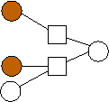
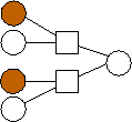
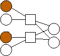
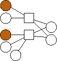
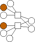
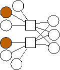
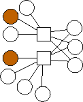
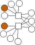
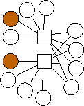
Second, there is a clear trend in the optimal graphs where m=2. That is that the data nodes are divided evenly into three classes: nodes with edges (0), nodes with edges (1), and nodes with edges (0,1). If n is not evenly divisible by three, then the first extra node has edges to 0 and 1, and the second extra node has an edge to 0. To show this pictorally, we picture them below in Figure 2. The shaded nodes are the coding nodes. We suspect that graphs of this form are optimal for all values of n but we have neither proved this nor quantified the overhead of these graphs.
 n=2 |
 n=3 |
 n=4 |
 n=5 |
 n=6 |
 n=7 |
 n=8 |
 n=9 |
 n=10 |
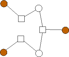
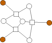
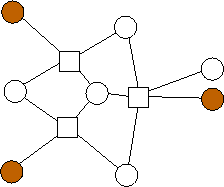
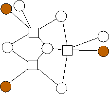
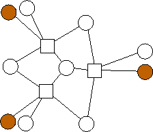
A similar trend emerges with m=3. Again, the n data nodes appear to be equally divided among the possible combinations of edge lists: {(0),(1),(2),(0,1),(0,2),(1,2),(1,2,3)}. However, unlike with m=2, where each additional value of n builds on the previous value's optimal graph in an identifiable pattern, in the limited graphs we have here, there is no such pattern. For example, the graph with n=4 builds on n=3 in a different way from the way in the analogous graph with n=11 builds on n=10. We will continue to explore these patterns.
 n=2 |
 n=3 |
 n=4 |
 n=5 |
 n=6 |
 n=7 |
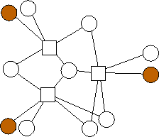 n=8 |
 n=9 |
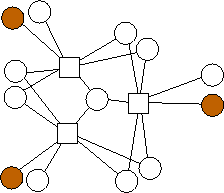 n=10 |
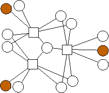 n=11 |
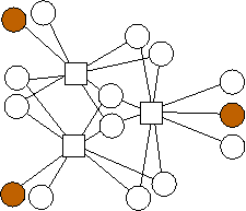 n=12 |
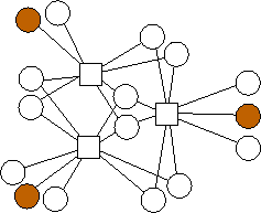 n=13 |
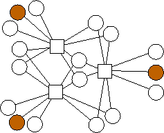 n=14 |
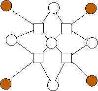
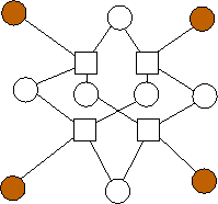
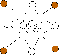
In Figure 4, we show the optimal graphs with m=4. Unlike the graphs for m=3 and m=2, these graphs do not build upon one another. As before, the n nodes are divided "evenly" between the possible combinations of edges. However, the way in which graphs build upon one another is not clear.
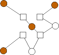 n=2 |
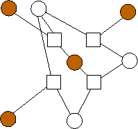 n=3 |
 n=4 |
 n=5 |
 n=6 |
 n=7 |
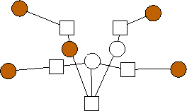
Finally, in Figure 5, we show the optimal graphs for m=5. Again, we will need to enumerate more graphs to discover whether there are interesting patterns to these optimal graphs.
 n=2 |
 n=3 |
When we start, we set all right-hand nodes to zero, and leave the values of all left-hand nodes blank.
To decode, we define two operations on graphs: assigning a value to a node, and downloading a node. Both operations are defined only on left-hand nodes. We start with the former. Given a left-hand node li, when the value of that node becomes known, it should be assigned. When it is assigned, for each right-hand node rj to which li is connected, rj's value is set to the exclusive-or of its previous value and li's value, and then the edge (li,rj) is removed from the graph. If there are any right-hand nodes rj which now have only one incident edge, then the value of the left-hand node to which rj is connected may now be assigned to be the value of rj. Before assigning the value, however, the edge between that node and rj should be removed, and rj should also be removed from the graph. Note, assigning one node's value can therefore result in assigning many other nodes' values.
To download a node, if the node's value has already been assigned, then the node is simply removed from the graph. Otherwise, the value of the node is assigned to its downloaded value, and it is then removed from the graph.
When the values of all left-hand nodes have been assigned, the decoding process is finished.
Computing the overhead o(G) of graph G proceeds as follows. If all nodes have zero edges, then the overhead is zero. Otherwise, we simulate downloading each left-hand node of the graph, and compute the average overhead as the average of all simulations. When we simulate downloading a node li, we assign its value (if unassigned), and remove the node from the graph. We are then left with a residual graph, R(G,li). We can recursively determine R(G,li)'s overhead. Then, the equation for determining a graph's overhead (if not zero), is:


This is a systematic code, where either node may be the data or coding bit. To decode, we first set r0's value to zero:

Then, suppose we download node l0, which has a value of 1. We assign its value by going through the following steps. We set its value to 1, then set r0's value to 0+1 = 1, and remove the edge (l0,r0), from the graph. Since r0 only has one incident edge now, which is to l1, we can assign l1's value to 1, and remove both the edge (l1,r0) and node r0 from the graph. Finally, we remove l0 from the graph. Thus, the residual graph R(G1,l0) is:

And the decoding process is finished. If we download node l1, the process is similar, and the decoding process finishes. Thus, to compute the overhead of decoding graph G1, o(G1), it is:

Note, this is a graph that represents a residual graph of a download, where we already know l2's value, but it has not been downloaded yet. To decode, if we download either nodes l0 or l1, then we may determine the value of all nodes, and decoding is complete. If we download node l2, then we simply remove that node from the graph, and are left with graph G1 as a residual. Therefore, the overhead of decoding G2 is:

This is a simple systematic replication code, where l0 is the data bit, and l1 and l2 are the coding bits. To decode, when any of the three nodes is downloaded, the values of the other two may be assigned. Therefore, the overhead of G3 is:

This is the optimal systematic code for n=2,m=2 and l=5. The data nodes are l0 and l1, and the coding nodes are l2 and l3. To decode, we look at the residual graphs of downloading each of the left-hand nodes. Downloading l0 leaves us with a graph equivalent to G2, Downloading l1 leaves us with a graph equivalent to G3. Downloading l2 leaves us with a graph equivalent to G2, and downloading l3 leaves us with a graph equivalent to G3. Therefore, the overhead of decoding graph G4 is:
Note, that matches the overhead for the graph in the tables above.
We will continue our exhaustive techniques until the graph sizes prove intractable for our computational power. Heuristics for enumerating unique bipartite graphs, and for indexing data structures by graphs will prove helpful.
Our initial exploration has illustrated trends in optimal graphs for m=2 and m=3. We will continue to explore these trends, and attempt to prove optimality for these codes for all values of n.
Finally, our exploration should help us define classes of graphs for larger values of n and m, which may not have optimal performance (or for which optimality cannot be proven), but which have good performance when compared to other evaluations of similarly sized graphs. As with this technical report, we hope to present such graphs so that the systems community, currently without any reference besides the asymptotic (and patented) techniques of Luby et al, have a methodology for constructing and using good systematic parity-check codes.