CS202 Lecture notes -- Running Times

James S. Plank
Directory: /home/plank/cs202/Notes/Running_Time
Lecture notes: http://web.eecs.utk.edu/~jplank/plank/classes/cs202/Notes/Running_Time/index.html
Original notes: Fall, 2019
Last modified: Fri Nov 22 11:08:25 EST 2019

This set of lecture notes is in two parts. In the first, I go over an example of implementing a class in seven ways, using pretty much every data structure that we've learned in this class, and then evaluating the running time of each way. That is in the "Histogram Example" below.

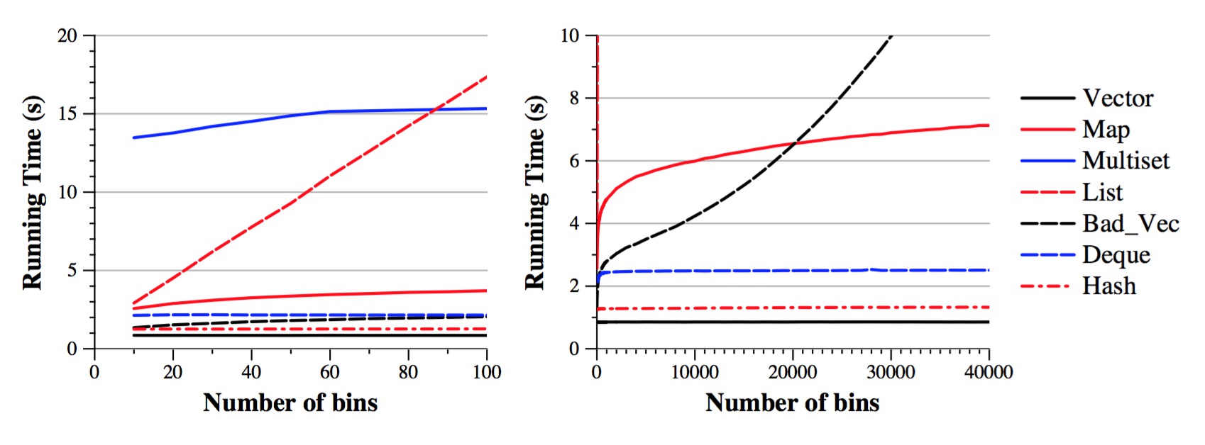After that, I go through a bunch of Topcoder problems, discuss their solutions (without implementing them), and then discuss the running times of the solution.

The goal of this set of lecture notes is to help you be able to take a problem and its solution, and derive the running time of the solution in terms of big-O.

Histogram Example

Please read the lecture notes on Using a Void * to implement a class. That lecture defines the Histogram class, some programs that use it, and one way to implement it.

I have implemented the class seven different ways, in seven different class implementations. They all work, but they all work differently. They provide an excellent review of the data structures that we've learned in this class. They are:

src/histogram_vector.cpp: This is the one described in the (void *) lecture. We maintain one vector, called Elts, such that Elts[i] contains the number of data points for bin i. We resize Elts when we need to insert a data point into a bin that is larger than Elts currently manages. When we implement Get_Data(), we traverse Elts and ignore bins that don't have any data.
src/histogram_map.cpp: Instead of a vector, we now have a map whose keys and vals are both integers. The keys are the bin numbers, and the vals are the number of data points in the bin. Insertion of a data point is straightforward: simply use the associative array feature of a map to increment a bin's val. If the bin wasn't in the map before, it will be in the map afterwards. Implementing Get_Data() simply traverses the map and creates the two vectors.
src/histogram_unordered_map.cpp: This is just like the map implementation above, except we use an ordered map instead. The only relevant code change is in Get_Data(). Since the data structure is unsorted, we create the bin_ids array by traversing the unordered_map, and then we sort the array. We then find the corresponding num_elts for each bin by finding it in the unordered_map.
src/histogram_multiset.cpp: Instead of using a map, we use a multiset, and whenever we call Add_Value(), we insert the bin of the value into the multiset. Get_Data() now traverses the multiset and counts up the number of times you see each bin.
src/histogram_list.cpp: Now we use a list, which tries to duplicate the functionality of the map above. The list stores bin/number pairs, and we keep it sorted. Add_Value() has to find the value, or where it needs to be inserted into the list. Then it updates the number, or adds the pair to the list. Get_Data() simply traverses the list to create the vectors.
src/histogram_bad_vec.cpp: As the name implies, this is a bad implementation. This works very similarly to the list implementation above, only now we maintain two vectors, Bins and Elts, which hold the bins and numbers respectively. We'll keep Bins sorted, and Elts[i] contains the number of data points for bin Bins[i]. Since Bins is a vector, we can use binary search to find a bin. Unfortunately, though, to insert a value into the bin, we have to make room for it, which can involve copying each element of Bins (and Elts) over one. In this implementation, Get_Data() is super-simple: you just copy Bins and Elts, because they are exactly what you want. This implementation is "bad", because similar to the list implementation, keeping Bins sorted is expensive.
src/histogram_deque.cpp: This implementation is very much like histogram_vector, except we use a deque instead of a vector. Moreover, instead of storing every bin starting from bin 0, we keep track of the minimum bin, and deque[index] stores the vals for bin index-minimum_bin. Now, when you add bins that are too big or too small, you either resize the deque (too big) or insert the proper number of zero bins to the front of the deque (too small). The insert operation has the same performance as resizing the deque. That's one of the things that makes deques attractive.
Because I know this will be confusing to some, let me simple show Minimum_Value and Elts after a few Add_Value() calls. We'll assume that the bin size is 10:
```
Action         Minimum_Value  Elts
-----------    -------------  ----
Start:               -1       {}
Add_Value(55)         5       { 1 }                      # We resize the deque by 1
Add_Value(71)         5       { 1, 0, 1 }                # We resize the deque by 2
Add_Value(58)         5       { 2, 0, 1 }
Add_Value(15)         1       { 1, 0, 0, 0, 2, 0, 1 }    # We insert four 0's to the front of the deque.
Add_Value(26)         1       { 1, 1, 0, 0, 2, 0, 1 }
```

(I have two other implementations -- src/histogram_hash.cpp, and src/histogram_hopscotch.cpp. You can ignore them.)

I'm not going to go through any of the code -- it's pretty straightforward, and it is commented. You'll note that all of the implementations use the (void *) as detailed in the (void *) lecture.

Basic Running Times

It's time for us to analyze running time, and memory consumption for the various implementation. I'm going to define the following quantities to help us:

n: This is the number of data items added to the histogram.
bins: This is the number of distinct bins that are in the histogram.
min: This is the minimum bin number.
max: This is the maximum bin number.

We're going to look at three quantities here -- two are running times, and one is memory consumption:

Create: This is the time to create the histogram from n elements. It is the time to perform n calls to Add_Value().
Get_Data: This is the time that it takes to call Get_Data() once you have created the histogram.
Space: This is the amount of memory consumed by the Histogram, once it has been created.

The following table summarizes these quantities for the seven implementations, all in terms of Big-O. I will explain how I arrived at these numbers after you see the table. It is a goal of CS202 to teach you to do these calculations yourself, so study up here, and make sure you understand everything in this table and explanation.

	Vector	Map	Unordered_map	Multiset	List	Bad_Vec	Deque
Create	O(n + max)	O(n log(bins))	O(n)	O(n log(n))	O(n bins)*	O(n log(bins) + bins²)	O(n + (max-min))
Get_Data	O(max)	O(bins)	O(bins log(bins))	O(n)	O(bins)	O(bins)	O(max-min)
Space	O(max)	O(bins)	O(bins)	O(n)	O(bins)	O(bins)	O(max-min)

Explanation for the vector implementation

Create: When you see a sum in a Big-O calculation, you can read it as "either-or, depending on which one is bigger." In this case, the performance is either O(n) or O(max), depending on which one is bigger. For example, if I insert 10,000 items that are all in bin 0, then the performance is O(n), because the vector resizing is minimal. However, if I insert one item into bin 1,000,000, then I have to create a vector with 1,000,001 elements, and the performance is O(max).

Get_Data: The vector has max elements, so traversing it is O(max). The size of the two resulting vectors will be bins, but clearly bins ≤ max. That is why it is O(max).

Space: The space is the size of the vector, which is max elements.

Explanation for the map implementation

Create: You are performing n find operations on the map, and bins insertions. The maximum size of the map is bins elements. Once the map starts filling up, each find and insert will be O(log(bins)), so the total running time is O(n log(bins)).

You may wonder -- shouldn't it be O(n log(bins) + bins log(bins))? That would account for the n find operations and the bins insertions. The answer is no. Why? because bins is clearly less than or equal to n. So (bins log(bins)) is less than or equal to (n log(bins)). Remember from our discourse on Big-O that constant factors don't matter with Big-O:

O(n log(bins) + bins log(bins)) ≤ O(2n log(bins)) = O(n log(bins)). This is why the answer is O(n log(bins)).

Get_Data: The map has bins elements, so traversing it is O(bins).

Space: The space is the size of the map, which is bins elements. Maps are implemented as balanced binary trees, and a tree with bins nodes consumes O(bins) space. Now, the map with bins elements is a lot bigger than a vector with bins elements, because the vector is very space efficient. However, they are both O(bins), because constant factors don't matter with Big-O.

Explanation for the unordered_map implementation

Create: You are performing n find operations on the unordered_map, and bins insertions. Because unordered_maps are implemented with resizable hash tables, each of these operations is O(1). So creation is O(n).

Get_Data: The unordered_map has bins elements, so traversing it to create bin_ids is O(bins). Sorting bin_ids is O(bins log(bins)). Then, each find() is O(1), so creating num_elts is O(bins). The total running time is therefore O(bins log(bins)).

Space: The space is the size of the unordered_map, which is O(bins).

Explanation for the multiset implementation

Create: You are performing n insertion operations on a multiset which will end up having n elements. This is O(n log(n)), plain and simple.

You may wonder -- when we're filling up the multiset, it has fewer than n elements, so why not something smaller than O(n log(n))? It's a good question, so let me prove to you that it is indeed O(n log(n)). Let's just consider the second half of the insertions. There are n/2 of these, and the multset contains at least n/2 elements in each insertion. So, the performance of those n/2 insertions is at least as big as O(n/2 log(n/2)). The constant factor doesn't matter, so this is O(n log(n/2)). And what is log(n/2)? It is log(n)-1. We know that O(x-1) is O(x), so O(log(n/2)) is O(log(n)). Therefore, the last n/2 insertions are O(n log(n)). The first n/2 insertions will be quicker than the second n/2, so they are less than O(n log(n)). So the n insertions are indeed O(n log(n)).

Get_Data: The multiset has n elements, so traversing it is O(n).

Space: The space is the size of the multiset, which is n elements.

Explanation for the list implementation

Create: You are performing n find operations on a list which will end up having bins elements. On average, each find operation has to traverse half of the list, so this is O(n*bins) for the find operations. The insertion operations are O(1), because this is a linked list. Thus, the insertions cost O(bins), which is clearly less than O(n*bins). For that reason, the total cost is O(n*bins).

Get_Data: The list has bins elements, so traversing it is O(bins).

Space: The space is the size of the list, which has bins elements.

Explanation for the bad vector implementation

Create: You are performing bins insertions, and n find operations. Since the find operations use binary search, each of them will be O(log(bins)). That's pretty cheap. The insertions on the other hand, have to move half of the vector elements, on average, to make room for the new bin. That's O(bins) for each bin, yielding O(bins²). We add the two quantities, because there may be times where O(n log(bins)) is greater than O(bins²), and vice versa.

Get_Data: The vectors have bins elements, so copying them is O(bins).

Space: The space is the size of the vectors, which is bins elements each. O(2*bins) is, of course, O(bins).

Explanation for the deque implementation

Create: This is very much like the vector implementation, only now, instead of having max elements, there are (max-min). We add n, because, like the vector implementation, this is an "either-or" situation.

Get_Data: The deque has (max-min) elements, so traversing it is O(max-min).

Space: The space is the size of the deque.

(If you want an explanation of the hash table implementation, look back before May, 2023 in the git repository).

Empirical Evaluation

Armed with this knowledge, we should be able to predict which implementation will do well in which scenario. For example, if I feed the values 0 and 100,000,000 into data_to_histogram, then n and bins are both equal to two, which is tiny. However, max, (max-min) and ts are comparatively large. For that reason, I expect the following:

Map, multimap, list and bad_vec will all perform well.
Hash will be slower.
Vector and deque will be the slowest.

Let's confirm:

UNIX> time sh -c "echo 0 100000000 | bin/dth_vector 1"            # Vector = 1 second
       0        1
   1e+08        1
1.008u 0.114s 0:01.12 99.1%	0+0k 0+0io 0pf+0w
UNIX> time sh -c "echo 0 100000000 | bin/dth_map 1"               # Map = negligible
       0        1
   1e+08        1
0.002u 0.003s 0:00.00 0.0%	0+0k 0+0io 0pf+0w
UNIX> time sh -c "echo 0 100000000 | bin/dth_unordered_map 1"     # Unordered_map = negligible
       0        1
   1e+08        1
0.004u 0.005s 0:00.01 100.0%	0+0k 0+0io 0pf+0w
UNIX> time sh -c "echo 0 100000000 | bin/dth_multiset 1"          # Multiset = negligible
       0        1
   1e+08        1
0.002u 0.004s 0:00.01 0.0%	0+0k 0+0io 10pf+0w
UNIX> time sh -c "echo 0 100000000 | bin/dth_list 1"              # List = negligible
       0        1
   1e+08        1
0.002u 0.003s 0:00.00 0.0%	0+0k 0+0io 0pf+0w
UNIX> time sh -c "echo 0 100000000 | bin/dth_bad_vec 1"           # Bad_Vec = negligible
       0        1
   1e+08        1
0.002u 0.003s 0:00.00 0.0%	0+0k 0+0io 0pf+0w
UNIX> time sh -c "echo 0 100000000 | bin/dth_deque 1"             # Deque = 2 seconds
       0        1
   1e+08        1
2.009u 0.147s 0:02.16 99.0%	0+0k 0+0io 0pf+0w
UNIX>

Let's use src/range_tester.cpp to test some other scenarios. Let's remind ourselves how it works:

UNIX> bin/range_vector
usage: range_tester bin_size n low high seed print(Y|N)
UNIX>

How about this: Let's insert 10,000,000 data points and modify the maximum values of the data points so that we modify the number of bins. You can see below that if we specify high as one, we get one bin, and if we specify high as 100,000, we get 100,000 bins:

UNIX> bin/range_vector 1 10000000 0 1 5 Y            # Here there's just one bin.
       0  10000000
Time for Create:     0.234
Time for Get_Data:   0.000
UNIX> bin/range_vector 1 10000000 0 100000 5 Y | wc  # Here there are 100,000 bins.
  100002  200008 1800054                             # (There are two lines for the timings)
UNIX> bin/range_vector 1 10000000 0 100000 5 N       # The O(n) part of Create dominates.
Time for Create:     0.276
Time for Get_Data:   0.005
UNIX>

Let's run an experiment. For each of the implementations, I vary the number of bins, and plot the time to add 10,000,000 values. I run over ten tests for each data point, and average the results. This is on a mid-grade Linux box.

Experiment to show the effect of modifying the number of bins when inserting 10,000,000 random elements

Let's see how this jibes with our understanding of the running times:

The vector, deque and hash implementations look like flat lines. That makes sense, because each of their Big-O equations is O(n + x), and in each case, n is greater than x. In our experiments, we hold n constant. That's why the lines are flat.

We can also conclude that vectors are more efficient data structures than deques. Let me quote from https://en.cppreference.com/w/cpp/container/deque:

"As opposed to std::vector, the elements of a deque are not stored contiguously: typical implementations use a sequence of individually allocated fixed-size arrays, with additional bookkeeping, which means indexed access to deque must perform two pointer dereferences, compared to vector's indexed access which performs only one."

The hash implementation is indeed fast, but it still performs more work than the vector implementation. It is slower by a factor of roughly 1.7. I surmised that compiler optimization might shrink that gap, but when I compiled both vector and hash with compiler optimization, it sped both of them up by more than a factor of two; however, the hash implementation was still 1.7 times slower.

The map implementation is slower in two ways -- Big-O and base implementation. Neither of these should come as a surprise to you. First, we definitely expect O(n log(bins)) to be slower than O(n). At the right edge of the graph above, bins is 40,000, which makes log(bins) roughly 15. That's significant, and the graph shows it.

What do you think of the shape of the map curve? Does it look like n log(bins) to you? Well, remember that we're holding n constant, so we should expect the curve to look like log (bins), and indeed it does. I like it when things make sense.

Let's look at two sets of timings:

Implementation:      bins=10         bins=40,000
---------------      -------         -----------
vector                0.86 s            0.85 s  
map                   2.57 s            7.12 s  
ratio map/vector      2.99              8.38

The log of 10 is 3.32 and the log of 40,000 is 15.28. So, the table above shows us that the map implementation is proportionally worse than the vector implementation when the number of bins is small (otherwise, we'd expect the ration when bins equals 40,000 to be 15). Can we make sense of that? Yes -- what I surmise is that when you are calling find() on the map, its performance is (x + log(bins)), where x is some startup costs (maybe a few "if" statements). When bins is small, the x term is significant. As bins grows, it becomes less significant.

Those other implementations are comparatively really bad. This is demonstrated in both the Big-O and in the graphs. The multiset is horrible, but we should expect it from the Big-O: The log of 10,000,000 is 23.26, so the performance of the multiset is on par with expectations.
The list implementation's curve looks like a straight line, which also matches expectations. It's Big-O equation is O(n * bins), and we're holding n constant, so we should expect a straight line!
The "bad" vector implementation has a Big-O of O(n log(bins) + bins²). So, when we hold n constant, we expect the quadratic term to dominate, and indeed that curve looks quadratic.
Question: Why is the bad_vec curve better than the list's curve, when O(n*bins) is faster than O(bins²)? (remember, we're holding n constant? Because the list implementation is performing O(bins) for every Add_Value() call, due to its linear lookup of the value. The bad_vec implementation performs O(log(bins)) for every Add_Value() call, because it uses binary search to find the value, and only does an O(bins) operation when it has to insert a new value. When bins is 40,000, the ratio of insertions to finds is 40,000/10,000,000, or 0.004. This is why the bad_vec implementation is faster than the list implementation -- it does the slow operation very infrequently, while the list operation does it at every Add_Value() call.
Question: If we keep increasing the number of bins, will the bad_vector implementation eventually become slower than the list implementation? Well, the gap will keep closing, but in reality, the bad_vec implementation never becomes slower (try the shell script in scripts/list_vec.sh). This is because we can't have more than n bins, so we can't keep increasing the bin size until the O(bins²) term becomes bigger than O(n*bins).

So, which implementation is best?

It depends. They all have plusses and minuses. I think that if I were writing a production implementation of this that *had* to work well in all cases, I would use the unordered_map addition to the STL (in C++11). That's a resizable hash table. On Get_Data(), I would store key/val pairs in one vector and then sort the vector with the STL's sort(), providing my own comparison function on pairs. I'll write this someday.

Topcoder Problems with Running Time Analyses

The analyses accompany the individual problem writeups: