Jgraph Chess Example

Evan Ezell
Directory: /home/plank/cs494/Notes/Jgraph
Original Creation: December, 2019

Note from Dr. P -- if you're on a Mac, this code will have issues, because Mac's ignore case with filenames. So "p.jpg" and "P.jpg" are identical. I've fixed the pictures for this web page, but if you're using the code, keep it in mind.

While taking Dr. Plank's Advanced Programming and Algorithms course in the Fall of 2019 I became fascinated with jgraph. The main reason I was fascinated with jgraph had to do with my love for Latex. Since jgraph can be converted to postscript, and postscript can be embedded in Latex, it is easy to create great graphics for research papers - and presentations with the Latex document class beamer. Because postscript uses vector graphics, you get no loss in quality which typically happens when trying to cram some jpeg in a paper column or presentation slide.

Following the semester, I decided to create jgraph chess graphics and an accompanying program to setup chess positions. First of all, the reasoning for doing this is my love for chess. Secondly, creating good chess graphics is important if I ever decide to create a chess writeup or presentation. The number of bad chess graphics that publishers still produce is astonishing to me. There are often negative reviews on a chess book just because of its poor quality in chessboard graphics.

It should be noted that there is a chessboard Latex package developed by Ulrike Fischer that is much more complete. The link to that package is https://ctan.org/pkg/chessboard. I developed the jgraph chess example as a use case to show the effectiveness of jgraph, not to compete with Fischer's package.

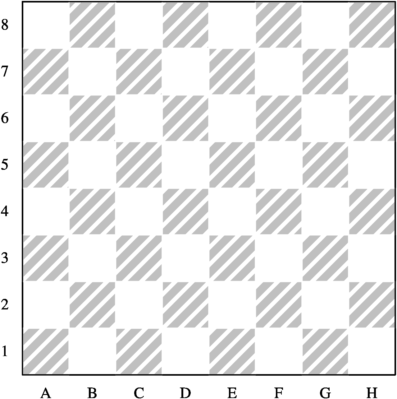
Creating the Chessboard

First, let's walk through creating a chessboard in jgraph. A standard chessboard has 64 squares - 8 rows known as ranks and 8 columns known as files. Ranks are numbered 1 through 8. Files are lettered A through H. The board is essentially a grid. Each square is uniquely specified by its file and rank, respectively.

(* chess board *)
newgraph

(* files *)
xaxis min 0.5 max 8.5 no_draw_axis
no_grid_lines no_draw_hash_marks no_auto_hash_labels
    hash_label at 1 : A
    hash_label at 2 : B
    hash_label at 3 : C
    hash_label at 4 : D
    hash_label at 5 : E
    hash_label at 6 : F
    hash_label at 7 : G
    hash_label at 8 : H

(* ranks *)
yaxis min 0.5 max 8.5 no_draw_axis
no_grid_lines no_draw_hash_marks no_auto_hash_labels
    hash_label at 1 : 1
    hash_label at 2 : 2
    hash_label at 3 : 3
    hash_label at 4 : 4
    hash_label at 5 : 5
    hash_label at 6 : 6
    hash_label at 7 : 7
    hash_label at 8 : 8

(* dark squares *)
shell : echo "" | awk '{\
    for (rank = 1; rank <= 8; rank++) { \
        if (rank % 2 == 0) file = 2; \
        else file = 1; \
        for (; file <= 8; file += 2) { \
            printf("newline poly gray 1 ppattern estripe 45 pfill .7 pts "); \
            printf("%f %f %f %f %f %f %f %f\n", \
                file - .5, rank - .5, \
                file + .5, rank - .5, \
                file + .5, rank + .5, \
                file - .5, rank + .5); \
        } \
    } \
}'

(* border *)
newline pts 0.5 0.5 0.5 8.5 8.5 8.5 8.5 0.5 0.5 0.5

Notice how I automatically generated the dark squares instead of laboriously brute forcing each square. Because jgraph allows you to execute a sh command using the ``shell'' keyword, we can create all of our squares via another language and embed this in our jgraph code for readability. I chose to create the dark squares using awk (see Dr. Plank's Awk Lecture). I like awk because it reads like C, but you can use whatever language you want to get the job done. I use this same technique to generate chess pieces (see section Creating Chess Pieces).

Also, to make things simpler, I chose to have each square be a 1 x 1 square with the xaxis and yaxis going from 0.5 to 8.5. This will allow us later to specify piece placement by putting them on their exact row and column. This makes writing a program to generate piece locations easier.

Creating Chess Pieces

Similar to the football (fbf.jgr) example from Dr. Plank's notes, we want to create encapsulated postscript (eps) marks to be used with our chessboard. First, I created all of the chesspieces in jgraph. Let's go through a few examples:

(* white chess pawn *)
newgraph
xaxis min 0 max 10 nodraw
yaxis min 0 max 10 nodraw

(* pawn base *)
newline bezier poly pfill 1 linethickness 10 pts
  0 0 2.5 0 7.5 0 10 0
    10 2 8 2 6 4
    5.5 4 4.5 4 4 4
    2 2 0 2 0 0

(* pawn center circle *)
newline poly pfill 1 linethickness 10 pts
    shell : echo "" | awk '{ \
        pi = atan2(0, -1); \
        for (i = 0; i <= 360; i += 1) { \
            printf(" %f %f",2*sin(i*pi/180)+5,2*cos(i*pi/180)+6); \
        } printf("\n") }'

(* pawn top circle *)
newline poly pfill 1 linethickness 10 pts
    shell : echo "" | awk '{ \
        pi = atan2(0, -1); \
        for (i = 0; i <= 360; i += 1) { \
            printf(" %f %f",1*sin(i*pi/180)+5,1*cos(i*pi/180)+9); \
        } printf("\n") }'

Above is a white chess pawn. This white pawn is made up of three simple elements: the base, the center circle, the top circle. The base can be described as a jgraph bezier polygon. You will notice there are straight lines in this polygon. I just specify a straight line by putting the two bezier control points collinearly between the endpoints. I fill the polygon with white (pfill 1) so that when the piece is on a dark square we do not see the square background in the middle of the piece. After we have the base, the head of the pawn is two circles. While I could have worked out each individual point along the circles, it is much easier to let awk do the work for us.

We can easily alter the white pawn to be a black pawn by changing the pfill to 0 of each of the three polygons. The black pawn looks as follows:

(* black chess pawn *)
newgraph
xaxis min 0 max 10 nodraw
yaxis min 0 max 10 nodraw

(* pawn base *)
newline bezier poly pfill 0 linethickness 10 pts
  0 0 2.5 0 7.5 0 10 0
    10 2 8 2 6 4
    5.5 4 4.5 4 4 4
    2 2 0 2 0 0

(* pawn center circle *)
newline poly pfill 0 linethickness 10 pts
    shell : echo "" | awk '{ \
        pi = atan2(0, -1); \
        for (i = 0; i <= 360; i += 1) { \
            printf(" %f %f",2*sin(i*pi/180)+5,2*cos(i*pi/180)+6); \
        } printf("\n") }'

(* pawn top circle *)
newline poly pfill 0 linethickness 10 pts
    shell : echo "" | awk '{ \
        pi = atan2(0, -1); \
        for (i = 0; i <= 360; i += 1) { \
            printf(" %f %f",1*sin(i*pi/180)+5,1*cos(i*pi/180)+9); \
        } printf("\n") }'

All of the other chess pieces were generated in a similar manner. The images of the resulting pieces are below.

	White Pieces	Black Pieces
Pawn
Bishop
Knight
Rook
Queen
King

Putting it all together

Now that we have postscript pieces. We can embed them as marks, placing them on the chessboard. For example, if we want to create the inititial chess position seen at the beginning of a match, we might do the following. Here is the jgraph code and resulting image:

(* chess board *)
newgraph

xaxis min 0 max 80 hash 10 mhash 0
grid_lines no_draw_hash_marks no_auto_hash_labels
    hash_label at 5  : A
    hash_label at 15 : B
    hash_label at 25 : C
    hash_label at 35 : D
    hash_label at 45 : E
    hash_label at 55 : F
    hash_label at 65 : G
    hash_label at 75 : H

yaxis min 0 max 80 hash 10 mhash 0 
grid_lines no_draw_hash_marks no_auto_hash_labels
    hash_label at 5  : 1
    hash_label at 15 : 2
    hash_label at 25 : 3
    hash_label at 35 : 4
    hash_label at 45 : 5
    hash_label at 55 : 6
    hash_label at 65 : 7
    hash_label at 75 : 8

(* print dark square background *)
shell : echo "" | awk '{ \
    for (rank = 0; rank < 8; rank++) { \
        if (rank % 2 == 0) file = 0; \
        else file = 1; \
        for (; file < 8; file += 2) { \
            printf("newline poly ppattern estripe 45 pfill .8 pts ");\
            printf("%d %d %d %d %d %d %d %d\n",\
                file * 10, rank * 10, \
                file * 10 + 10, rank * 10, \
                file * 10 + 10, rank * 10 + 10, \
                file * 10, rank * 10 + 10); \
        } \
    } \
}'

newcurve eps ps_pieces/r.ps marksize 8 8 pts 5 75
newcurve eps ps_pieces/n.ps marksize 8 8 pts 15 75
newcurve eps ps_pieces/b.ps marksize 8 8 pts 25 75
newcurve eps ps_pieces/q.ps marksize 8 8 pts 35 75
newcurve eps ps_pieces/k.ps marksize 8 8 pts 45 75
newcurve eps ps_pieces/b.ps marksize 8 8 pts 55 75
newcurve eps ps_pieces/n.ps marksize 8 8 pts 65 75
newcurve eps ps_pieces/r.ps marksize 8 8 pts 75 75
newcurve eps ps_pieces/p.ps marksize 8 8 pts 5 65
newcurve eps ps_pieces/p.ps marksize 8 8 pts 15 65
newcurve eps ps_pieces/p.ps marksize 8 8 pts 25 65
newcurve eps ps_pieces/p.ps marksize 8 8 pts 35 65
newcurve eps ps_pieces/p.ps marksize 8 8 pts 45 65
newcurve eps ps_pieces/p.ps marksize 8 8 pts 55 65
newcurve eps ps_pieces/p.ps marksize 8 8 pts 65 65
newcurve eps ps_pieces/p.ps marksize 8 8 pts 75 65
newcurve eps ps_pieces/P.ps marksize 8 8 pts 5 15
newcurve eps ps_pieces/P.ps marksize 8 8 pts 15 15
newcurve eps ps_pieces/P.ps marksize 8 8 pts 25 15
newcurve eps ps_pieces/P.ps marksize 8 8 pts 35 15
newcurve eps ps_pieces/P.ps marksize 8 8 pts 45 15
newcurve eps ps_pieces/P.ps marksize 8 8 pts 55 15
newcurve eps ps_pieces/P.ps marksize 8 8 pts 65 15
newcurve eps ps_pieces/P.ps marksize 8 8 pts 75 15
newcurve eps ps_pieces/R.ps marksize 8 8 pts 5 5
newcurve eps ps_pieces/N.ps marksize 8 8 pts 15 5
newcurve eps ps_pieces/B.ps marksize 8 8 pts 25 5
newcurve eps ps_pieces/Q.ps marksize 8 8 pts 35 5
newcurve eps ps_pieces/K.ps marksize 8 8 pts 45 5
newcurve eps ps_pieces/B.ps marksize 8 8 pts 55 5
newcurve eps ps_pieces/N.ps marksize 8 8 pts 65 5
newcurve eps ps_pieces/R.ps marksize 8 8 pts 75 5

The jgraph board code is exactly the same as the empty board shown previously; we just have to specify where we would like to place the pieces. For example, the white king is specified by the following code:

newcurve eps ps_pieces/K.ps marksize 8 8 pts 45 5

While typing this everytime works, it can be quite tedious to try and calculate the location of where you want to place each piece, especially when most all the pieces are left on the board. We probably want a more intuitive way to specify piece locations.

Generating a specific board in a more intuitive way

In chess there are several different formats one can use to specify a particular board and/or the current state of the game. The International Chess Federation (FIDE) requires players to write down their moves using standard algebraic notation. Another common notation is the Forsyth-Edwards Notation (FEN), which describes the current state of a game. As an example here, we will use a format similar to the GNU Chess (https://www.gnu.org/software/chess/) board output in terminal mode.

The format goes like this. Each square's state is specified by a character. Below is a chart of all the possible square states and their corresponding character representation.

Character	Square State
.	empty square
P	white pawn on square
B	white bishop on square
N	white knight on square
R	white rook on square
K	white king on square
Q	white queen on square
p	black pawn on square
b	black bishop on square
n	black knight on square
r	black rook on square
k	black king on square
q	black queen on square

Each row of the board is specified by eight of the above characters and is terminated by a newline. The board is specified from the white player's perspective. For example, the initial board would be specified by the following:

rnbqkbnr
pppppppp
........
........
........
........
PPPPPPPP
RNBQKBNR

This representation will make it much easier to specify a particular board. We now need a way of converting this representation to a jgraph chess board with the pieces located in their corresponding positions. I have written a C program (gen_chessboard.c), which will translate the board for us.

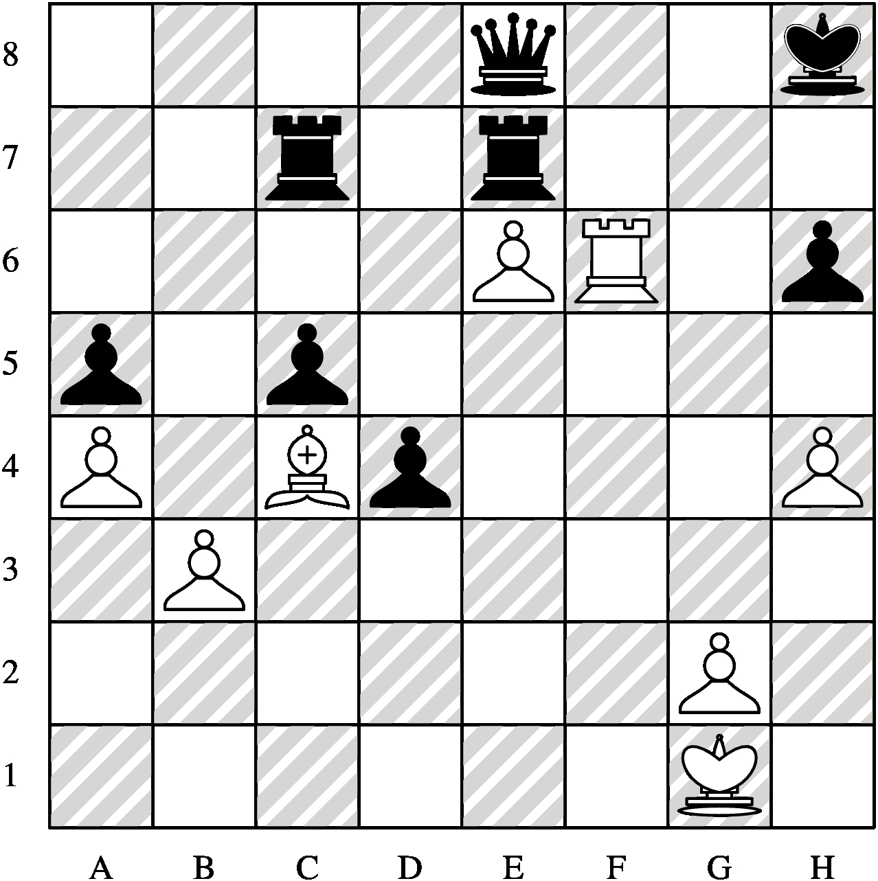
Final Example

Let's say we want to specify Fischer versus Spassky, Game 6 of the 1972 World Chess Championship, widely known as the Match of the Century, taking place during the Cold War. The final board of the game is in the file example_boards/fischer_spassky_game6_1972.txt and shown below:

....q..k
..r.r...
....PR.p
p.p.....
P.Bp...P
.P......
......P.
......K.

We want to convert this to a jgraph board. We can use our C program gen_chessboard. It can read the board directly off of stdin. In order to generate the board, we could run the following:

UNIX> cat example_boards/fischer_spassky_game6_1972.txt | ./gen_chessboard >fischer_spassky_game6_1972.jgr
UNIX> cat fischer_spassky_game6_1972.jgr
(* chess board *)
newgraph

xaxis min 0 max 80 hash 10 mhash 0
grid_lines no_draw_hash_marks no_auto_hash_labels
    hash_label at 5  : A
    hash_label at 15 : B
    hash_label at 25 : C
    hash_label at 35 : D
    hash_label at 45 : E
    hash_label at 55 : F
    hash_label at 65 : G
    hash_label at 75 : H

yaxis min 0 max 80 hash 10 mhash 0 
grid_lines no_draw_hash_marks no_auto_hash_labels
    hash_label at 5  : 1
    hash_label at 15 : 2
    hash_label at 25 : 3
    hash_label at 35 : 4
    hash_label at 45 : 5
    hash_label at 55 : 6
    hash_label at 65 : 7
    hash_label at 75 : 8

(* print dark square background *)
shell : echo "" | awk '{ \
    for (rank = 0; rank < 8; rank++) { \
        if (rank % 2 == 0) file = 0; \
        else file = 1; \
        for (; file < 8; file += 2) { \
            printf("newline poly ppattern estripe 45 pfill .8 pts ");\
            printf("%d %d %d %d %d %d %d %d\n",\
                file * 10, rank * 10, \
                file * 10 + 10, rank * 10, \
                file * 10 + 10, rank * 10 + 10, \
                file * 10, rank * 10 + 10); \
        } \
    } \
}'

newcurve eps ps_pieces/q.ps marksize 8 8 pts 45 75
newcurve eps ps_pieces/k.ps marksize 8 8 pts 75 75
newcurve eps ps_pieces/r.ps marksize 8 8 pts 25 65
newcurve eps ps_pieces/r.ps marksize 8 8 pts 45 65
newcurve eps ps_pieces/P.ps marksize 8 8 pts 45 55
newcurve eps ps_pieces/R.ps marksize 8 8 pts 55 55
newcurve eps ps_pieces/p.ps marksize 8 8 pts 75 55
newcurve eps ps_pieces/p.ps marksize 8 8 pts 5 45
newcurve eps ps_pieces/p.ps marksize 8 8 pts 25 45
newcurve eps ps_pieces/P.ps marksize 8 8 pts 5 35
newcurve eps ps_pieces/B.ps marksize 8 8 pts 25 35
newcurve eps ps_pieces/p.ps marksize 8 8 pts 35 35
newcurve eps ps_pieces/P.ps marksize 8 8 pts 75 35
newcurve eps ps_pieces/P.ps marksize 8 8 pts 15 25
newcurve eps ps_pieces/P.ps marksize 8 8 pts 65 15
newcurve eps ps_pieces/K.ps marksize 8 8 pts 65 5
UNIX> jgraph fischer_spassky_game6_1972.jgr >fischer_spassky_game6_1972.ps
The resulting board is below: