
| Figure 2.5: Recursive matrix layout in logical (algorithmic) and physical (main memory) views. |
To the Graduate Council:
I am submitting herewith a dissertation written by Piotr Rafal Luszczek entitled “Performance Improvements of Common Sparse Numerical Linear Algebra Computations.” I have examined the final electronic copy of this dissertation for form and content and recommend that it be accepted in partial fulfillment of the requirements for the degree of Doctor of Philosophy, with a major in Computer Science.
| Dr. Jack J. Dongarra |
| Major Professor |
| We have read this dissertation |
| and recommend its acceptance: |
| Dr. Allen Baker |
| Dr. Michael Berry |
| Dr. Victor Eijkhout |
| Accepted for the Council: |
| Dr. Anne Mayhew |
| Vice Provost and |
| Dean of Graduate Studies |
A Thesis
Presented for the
Doctor of Philosophy Degree
The University of Tennessee, Knoxville
Piotr Rafal Luszczek
May 2003
Acknowledgments
I would like to thank my advisor, Prof. Dongarra, for letting me first become his student and then for his guidance, mentorship and continuing support that made this research possible.
I am thankful to Profs. Baker, Berry, and Eijkhout for agreeing to serve on my graduate committee, providing me with helpful suggestions, and contributing to seamless cooperation.
In addition, I would like to express my appreciation to Profs. Langston and Raghavan who offered invaluable advices on technical issues that I was facing while working on this dissertation.
Also, the sponsorship of the National Science Foundation and the Department of Energy is acknowledged as this work was supported in part by the University of California Berkeley through subcontract number SA2283JB, as a part of the prime contract ACI-9813362 from the National Science Foundation; and by the University of California Berkeley through subcontract number SA1248PG, as a part of the prime contract DEFG03-94ER25219 from the U.S. Department of Energy.
Abstract
Manufacturers of computer hardware are able to continuously sustain an unprecedented pace of progress in computing speed of their products, partially due to increased clock rates but also because of ever more complicated chip designs. With new processor families appearing every few years, it is increasingly harder to achieve high performance rates in sparse matrix computations. This research proposes new methods for sparse matrix factorizations and applies in an iterative code generalizations of known concepts from related disciplines.
The proposed solutions and extensions are implemented in ways that tend to deliver efficiency while retaining ease of use of existing solutions. The implementations are thoroughly timed and analyzed using a commonly accepted set of test matrices. The tests were conducted on modern processors that seem to have gained an appreciable level of popularity and are fairly representative for a wider range of processor types that are available on the market now or in the near future.
The new factorization technique formally introduced in the early chapters is later on proven to be quite competitive with state of the art software currently available. Although not totally superior in all cases (as probably no single approach could possibly be), the new factorization algorithm exhibits a few promising features.
In addition, an all-embracing optimization effort is applied to an iterative algorithm that stands out for its robustness. This also gives satisfactory results on the tested computing platforms in terms of performance improvement. The same set of test matrices is used to enable an easy comparison between both investigated techniques, even though they are customarily treated separately in the literature.
Possible extensions of the presented work are discussed. They range from easily conceivable merging with existing solutions to rather more evolved schemes dependent on hard to predict progress in theoretical and algorithmic research.
The computer hardware industry (and its high performance branch in particular) continues to follow Moore’s law [122, 124] even though there exist skeptical opinions [158]. This development trend on the one hand makes the integrated circuits faster, but on the other hand, more complex and harder to use. At the same time, there exists an ever increasing demand from science and industry for yet higher computation rates – Grand Challenge problems [109, 121, 126, 127] and the interest in the Grid [72] exemplify the need. In a nutshell, this work shows a way of applying recent algorithmic advances in dense numerical linear algebra and matrix ordering optimizations in sparse computational kernels, namely direct and iterative codes.
The prevalent processor architecture for high performance computers has been Reduced Instruction Set Computer (RISC) and recently (for the second time in history) also Complex Instruction Set Computer (CISC) [44, 122] with introduction of increasingly powerful commodity desktop computers. Despite the differences between the two, when solving applied numerical linear algebra problems they benefit from similar optimization techniques [51, 88] – those that are used in tuned versions of Basic Linear Algebra Subroutines (BLAS) [56, 163] and deliver a rather high percentage of theoretical peak performance [55]. Unfortunately, many interesting scientific and commercial problems cannot be formulated in terms of dense linear algebra kernels since that would require prohibitive amounts of storage and computational capacity. In effect, possible formulations are the main source of sparse matrices that have had customarily large dimensions because they commonly originate in discretizations of rather large multidimensional problems. A positive feature of sparse matrices is that relatively few entries that need to be considered during computations and while storing them. This has been taken advantage of in many ways, most commonly to reduce storage requirements. The computational efficiency suffers because intricate data structures do not match the execution patterns favored by modern Central Processing Units (CPU). Clearly, BLAS is for now the only way to achieve the levels of performance that are commonly advertised by hardware vendors. To address this problem, it is necessary to consider how a contemporary CPU handles floating point (FP) data, how BLAS use this information, and why sparse computations fail in this respect.
On modern CPUs, the two major issues that hinder efficient calculations of sparse codes, as opposed to dense codes, are an extra demand for memory bandwidth and additional fixed point calculations. Both of these are directly related to sparse data storage schemes which require transfer and processing of integer data [156]. The former may be addressed in a novel way – by use of recursion [53, 54]. It was possible because of recent introduction of recursion-based formulation of matrix decomposition algorithms [67, 95, 157] that reduce the memory bus traffic. In addition, if the recursive LU algorithm is combined with a recursive layout [93] then the resulting code is superior to any known software techniques as shown later on. This is chosen as the premise for possible application in a direct sparse solver. The latter issue of integer arithmetic may be addressed with direct use of BLAS. This, however, will require reformulating FP computations, but there exist ways to do so and they will be elaborated on later. The point needs to be stressed here that the transfer of data that describes the sparsity structure (not present in dense computations) is more important than the extra calculations on such data because of the widening gap between the processor and system bus speeds – a fact illustrated quite well by the ratio of performance of BLAS xGEMV and xGEMM routines as presented in section 4.2.
A quick argument in favor of recursive formulation of a computational task may easily be made with a simple example of the Fibonacci series. The traditional way of defining the Fibonacci series is this:
|
This is a, so called, tail recursion. In order to calculate a single element of the series all preceeding elements have to be calculated first. It may be (rather easily) proven that the following definition is an equivalent one:
|
The latter formulation uses a divide and conquer recursion and even intuitively should be faster. The intuition proves correct in practice because the latter formulation is typically orders of magnitude faster. The former formulation is in a sense analogous to the LU decomposition method used in LINPACK [46] – a single column of the matrix is factored at a time. The latter formulation of the Fibonacci series corresponds the aforementioned recursive LU factorization – at any given point of the algorithm both halves of the matrix are processed recursively.
The are more examples of rather elegant use of recursion to formulate a superior algorithm. To name the some of them, the Fast Fourier Transform (FFT) [123] and Nested Disection [76] algorithms should be mentioned. In these cases, the divide and conquer recursion was successfully used to reduce the computational cost of a computational task.
In practice, direct methods could fail for two main reasons: prohibitive amount of storage requirements due to fill-in and/or extremely long factorization time (again due to fill-in). In such cases, an iterative method is a viable solution. On one hand, it does not incur fill-in and on the other (if matrix properties permit) executes far less FP operations in comparison with a direct method. However, iterative methods are known for lack of robustness, i.e. might not converge for a well-conditioned matrix. It is less of a problem with emergence of techniques such as the Bi-CGSTAB [161] method designed in a sense for unsymmetric matrices. Once the choice of the method has been made, performance optimization options need to be considered. As it was the case in direct methods, integer indices are the main performance concern. A different optimization goal is striven here as the dominant operation is matrix-vector multiplication (contrasting with matrix-matrix multiplication for direct codes). Consequently, a different approach must be taken – the one that optimizes system bus utilization and takes advantage of RISC architectures for relatively small dense structures present in sparse matrices – be it short vectors or elongated rectangular matrices. In particular, in such a setting BLAS cannot be considered to leverage hardware’s high computational rate as the function call overhead cannot be offset by possible performance gains.
The main objective of this work is to improve solution time of the following system of linear equations:
| Ax = b, (1.1) |
where A is a n by n real matrix (A∈ ℝn× n), and x and b are n-dimensional real vectors (b, x∈ℝn). The values of A and b are known and the task is to find x satisfying (1.1). It is assumed that the matrix A is large (of order commonly exceeding ten thousand) and sparse, in other words, there are enough zero entries in A that it is beneficial to use special computational methods to factor the matrix rather than to use a dense code. There are two common approaches that are used to deal with such a case, namely, iterative [146] and direct methods [58].
Iterative methods, in particular techniques based on Krylov subspace such as the Conjugate Gradient [97] algorithm, are the methods of choice for the discretizations of elliptic or parabolic partial differential equations where the resulting matrix is often guaranteed to be positive definite or close to it. However, when the linear system matrix is strongly unsymmetric or indefinite, as is the case with matrices originating from systems of ordinary differential equations or the indefinite matrices arising from shift-invert techniques in eigenvalue methods [41], one has to revert to direct methods [58]. For such methods, this study analyzes how the recursive formulation of the LU factorization algorithm can be efficiently applied to sparse matrices. It involves consideration of a matrix ordering scheme applied prior to factorization. Various schemes for sparse matrix storage are considered to exploit most commonly used computer architectures and existing software for matrix computations.
An attractive meeting point between direct and iterative methods is preconditioning [19]. In a sense, it addresses shortcomings of both approaches. Common causes of failure for direct methods are excessive storage requirements to accommodate fill-in or prohibitive amount of FP operations. On the other hand, iterative methods (especially non-stationary ones) are quite capricious when it comes to matrix spectrum considerations. Preconditioning fits perfectly in such a situation. It allocates space for a closely controlled amount of fill-in and consequently has predictable computational complexity. L and U factors resulting from incomplete LU preconditioning are often less numerically accurate than those from the proper Gaussian elimination process, but are good enough to bring the iteration matrix close to the identity matrix. As the name – incomplete LU – indicates, there is a notion of incompleteness involved in the methods that are used in preconditioning. This favorably coincides with the fact that the recursive LU factorization for sparse matrices does not perform pivoting – a possibly incomplete solution for some matrices but quite likely sufficient for the purposes of applications involving iterative methods.
This study is concerned with application of recursion to direct methods, which have a drawback of incurring fill-in in the factored matrix which, in turn, may prohibit factorization of large matrices due to excessive memory requirements. To increase the performance, the Level 3 BLAS have to be used. This places extra burden on the matrix ordering which has to fulfill one more requirement, i.e., it has to introduce dense sub-matrices in the original matrix structure. This, again, may not be possible for certain types of matrices. Thus, the study aims at optimizing performance for as many types of matrices as possible with the provision of less satisfactory results for remaining matrices.
Another decision made early in the development process was to not include pivoting in the recursive sparse LU code. Obviously it simplifies the algorithm but simplification was not the only reason. There exist strong evidence [114, 115] that other techniques (mainly a form of equilibration [60]) provide enough countermeasures against excessive pivot growth during the factorization for most cases. However, if during the factorization a diagonal value occurs that is dangerously close to 0, it is dealt with techniques described later on (see section 2.5).
The iterative method research is limited to the unpreconditioned Bi-CGSTAB method. Other researchers have considered the use of multiple iterative methods [20]. In addition, even though preconditioning is an attractive option to increase robustness [19] and serves as an interesting conceptual bridge between a true direct code and a purely iterative method but consequently it poses new challenges which were decided to be left out of this effort. However, this research provides concepts, tools, and techniques to create a preconditioned iterative method.
Yet another constraint imposed on this research is the rather early maturity state of parallel implementations of the recursive LU code for dense matrices [106, 107]. Naturally, a high quality parallel dense recursive solver would be a perfect starting point for a parallel sparse recursive solver as it was the case in the sequential case. More thorough scalability considerations need to be provided prior to competing with existing sparse solvers for parallel machines. A contrasting argument is raised against including parallel iterative method techniques here – namely a rather interesting concepts were proposed by others [20, 63] which do not fit directly into the problem addressed by this writing.
Lastly, techniques specific to Vector Processing Units (VPU) are not included here as the processors traditionally have been addressing the problem of sparse computations with gather and scatter instructions and the optimizations considered here result in rather short (in VPU vernacular) vector lengths which quite certainly would not yield substantial benefits.
Given a system of linear equation denoted with
| Ax = b, (2.1) |
where A is a n by n real matrix (A∈ ℝn× n), and x and b are n-dimensional real vectors (b, x∈ℝn) the Gaussian elimination with partial pivoting [89] is performed to find a solution of (2.1). Most commonly, the factored form of A is given by means of matrices L, U, P and Q such that:
| LU = PAQ, (2.2) |
where:
A simple transformation of (2.1) yields:
| (PAQ)Q−1x=Pb, (2.3) |
which in turn, after applying (2.2), gives:
| LU(Q−1x)=Pb, (2.4) |
Solution to (2.1) may now be obtained in two steps:
|
and these steps are performed through so called forward and backward substitutions. The matrices involved in the substitutions are triangular and therefore solving (2.5) and (2.6) is faster than solving (2.1). More precisely, the most computationally intensive part of solving (2.1) is the LU factorization defined by (2.2). This operation has computational complexity of order O(n3) when A is a dense matrix, as compared to O(n2) for the substitution phase. Therefore, optimization of the factorization is the main determinant of the overall performance.
When both of the matrices P and Q of (2.2) are non-trivial, i.e. neither of them is an identity matrix, then the factorization is said to be using complete pivoting. In practice, however, Q is an identity matrix and this strategy is called partial pivoting which tends to be sufficient to retain numerical stability of the factorization, unless the matrix A is singular or nearly so [152]. Moderate values (κp≪є−1) of the condition number κp=||A−1||p ||A||p guarantee a success for a direct method as opposed to matrix norm and spectrum considerations required for iterative methods.
It is assumed that A is sparse, which may be formulated as
| n≤η(A)≪ n2, (2.7) |
where η(A) is the number of (structural) nonzero entries in A. Many authors avoid an explicit definition of sparsity in quantitative terms. It is commonly accepted, though, that the aim is for the amount of fill-in and computational complexity to be proportional to O(n)+O(η(A)) [51]. If the matrix A is sparse, it is important for the factorization process to operate solely on the non-zero entries of the matrix. However, new nonzero entries are introduced in the L and U factors which are not present in the original matrix A of (2.1). The new entries are referred to as fill-in and cause the number of non-zero entries in the factors (we use the notation η(A) for the number of non-zeros in a matrix) to be (almost always) greater than that of the original matrix A: η(L+U)≥η(A). The amount of fill-in can be controlled with the matrix ordering performed prior to the factorization and consequently, for the sparse case, both of the matrices P and Q of (2.2) are non-trivial. Matrix Q induces a column reordering that minimizes fill-in and P permutes rows so that pivots selected during the Gaussian elimination warrant numerical stability.
function xGETRF(matrix (Rn× n∋) A≡ [aij] i,j=1,…,n) begin for i = 2,…,n do begin aij:=1/ajj(aij−∑k=1j−1aikakj) j = 1,…,i − 1 aij:=(aij−∑k=1i−1aikakj) j = i,…,n end end
Figure 2.1: LU factorization function of a dense matrix A that uses Gaussian elimination and does not perform pivoting.
function xGETRF(matrix A∈ℝm× n) if (A∈ ℝm× 1) If the matrix has just one column. |ak1| := max1≤ i≤ n|ai1| Find a suitable pivot – equivalent to the Level 1 BLAS IxMAX. a11 :=: ak1 Exchange a11 with ak1. A := 1/a11 A Scale the matrix – equivalent to the Level 1 BLAS xSCAL. else begin k := min{m, n} k1 := ⌊ k/2 ⌋ m1 := m − k1 n1 := n − k1 Divide matrix A into four sub-matrices: A=[ ]
A1 1 A1 2 A2 1 A2 2 [ ]
ℝk1 × k1 ℝk1 × n1 ℝm1 × k1 ℝm1 × n1 xGETRF([ A11 A21 ]T) Recursive call. xLASWP([ A12 A22 ]T) Apply pivoting from the recursive call. A12 := L1(A11)−1 A12 Perform a lower triangular solve which is equivalent to the Level 3 BLAS xTRSM function. A22 := A22 − A21 A12 Compute the Schur’s complement which is equivalent to a matrix-matrix multiply performed by the Level 3 BLAS xGEMM function. xGETRF(A22) Recursive call. xLASWP([ A11 A21 ]T) Apply pivoting from the recursive call. end end.
Figure 2.2: Recursive LU factorization function of a dense matrix A equivalent to the LAPACK’s xGETRF function (partial row pivoting is performed).
Figure 2.1 shows the classical LU factorization code which uses Gaussian elimination. Rearrangement of the loops and introduction of blocking techniques can significantly increase performance rates achieved by this code [11, 40]. However, the recursive formulation of the Gaussian elimination shown in Figure 2.2 exhibits superior performance [95, 157]. It does not contain any looping statements and most of the floating point operations are performed by the Level 3 BLAS routines: xTRSM and xGEMM. These routines achieve near-peak Mflop/s rates on modern computers with deep memory hierarchy. They are incorporated in many vendor-optimized libraries, and also the ATLAS project [56, 163] automatically generates implementations tuned to specific platforms. Some properties of the recursive LU algorithm are established by the following theorems.
Theorems 1 and 2 compare the amount of memory traffic – called I/O for short – for LAPACK’s blocked implementation of LU factorization and the recursive one. The memory traffic that is being accounted for in the theorems is the one that takes place between the Level 1 cache (referred to as primary memory) and the rest of the memory hierarchy (most commonly Level 2 cache).
| IOMM(n,n,m)≤ | ⎧ ⎪ ⎪ ⎨ ⎪ ⎪ ⎩ |
|
| IOTS(m,m)≤ | ⎧ ⎪ ⎪ ⎨ ⎪ ⎪ ⎩ |
|
| IORP(n,m)≤2nm | ⎛ ⎜ ⎜ ⎜ ⎜ ⎝ |
| +logm | ⎞ ⎟ ⎟ ⎟ ⎟ ⎠ | +2n2(1+logm) |
| IOMM(t,r,s)≤ | ⎧ ⎪ ⎪ ⎨ ⎪ ⎪ ⎩ |
|
| IOTS(r,s)≤ | ⎧ ⎪ ⎪ ⎨ ⎪ ⎪ ⎩ |
|
| IORL(n,m)≥ | ⎧ ⎪ ⎪ ⎪ ⎪ ⎪ ⎨ ⎪ ⎪ ⎪ ⎪ ⎪ ⎩ |
|
| +2nm≥ |
| +2nm. |
Theorem 3 provides another insight into the superiority in performance exhibited by the recursive factorization. The theorem introduces quantity called area of the matrix operands passed to BLAS. Clearly, a BLAS subroutine references memory locations that hold matrix entries. Such references incur memory bus traffic which needs to be optimized since it is the bottleneck of the factorization. The theorem shows that the recursive algorithm is more optimal with respect to area of the matrix operands passed to BLAS.
| AR(mNB,nNB) = (((2+⌊logn⌋)n − 21+⌊logn⌋)m + f(n))NB2 |
| f(2k)=2k(k(1−2×2k) + 5(2k− 1))/4 |
| AR(nNB,nNB) = 2k−2(k(2k+1+1) + 5(2k− 1)]NB2. |
| AL(mNB,nNB) = ((n(n + 1)/2)(m − n/3 + 4/3) − m − 1)NB2. |
Finally, Lemma 1 and Theorem 4 show that asymptotically the recursive and iterative (loop-based) factorizations perform the same number of FP operations.
Proof Let FD denote divisions by pivot and FU – additions and multiplications during the update phase. The outer-product update version of the factorization will be used in the proof.
In each column, all entries below the diagonal need to be divided by the pivot element. And so there are m−1 divisions in the first column, m−2 in the second, and so on, until the nth column where there are m−n divisions. Thus:
|
There are n−1 updates (there is no update in the last column) – an update in column i (1≤ i≤ n−1) is an outer-product update which performs 2(m−i)(n−i) FP operations (it may be regarded as a xGEMM call with the third dimension equal to one). Thus:
|
And finally:
| FD+FU=mn2−n3/3−n2/2−n/6 |
Proof For simplicity, it is assumed that m and n are powers of 2. Let f(m,n) denote the number of FP operations in the recursive LU factorization of an m× n matrix. At each (other than a single column case) recursion level the following operations are performed:
Thus, the function f satisfies the following recursive equation:
| f(m,n)=f(m,n/2)+(n/2)3+2(n/2)2(m−n/2)+f(m−n/2,n/2) (2.8) |
Since for the proof only the high order terms are relevant then function f is of the form:
| f(m,n)=α mn2+β n3+γ m2n+δ m3 (2.9) |
Coefficients α, β, γ, and δ are determined by substituting equation (2.9) in equation (2.8):
|
To simplify, we immediately observe that:
| δ m3≡δ m3+δ m3⇒δ=0 |
Gathering “mn2 terms” yields:
| α mn2≡α mn2/4+mn2/2+α mn2/4−γ mn2/2 |
and thus:
| α=α/4+1/2+α/4−γ/2⇒α=1−γ. |
Similarly “n3 terms” give:
| β n3≡β n3/8+n3/8−n3/4−α n3/8+β n3/8+γ n3/8 |
so that:
| β=β/8+1/8−1/4−α/8+β/8+γ/8⇒β= |
| . |
To determine the value of γ the “initial condition” f(2,2)=2 is used, which is combined with (2.9): f(2,2)=8α+8β+8γ. This gives γ=0 and consequently β=−1/3 and α=1. Finally then (2.9) may be written as
| f(m,n)=mn2−n3/3. |
An alternative formulation of the recursive algorithm is proposed here and shown in Figure 2.3. Most notable difference is the lack of pivoting code and additional calls to Level 3 BLAS. Experiments show that this code performs equally well as the code from Figure 2.2. The experiments also provide indications that further performance improvements are possible, if the matrix is stored recursively [93]. A simplified but still recursive storage scheme is proposed and illustrated in Figures 2.4 and 2.5. This scheme causes dense square sub-matrices to be aligned recursively in memory which is a discrete mapping between one dimensional main memory and matrix entries that form a two dimensional array. The recursive algorithm from Figure 2.3 traverses the recursive matrix structure all the way down to the level of a single dense sub-matrix. At this point an appropriate computational routine is called (either BLAS or xGETRF). Depending on the size of the sub-matrices (referred to as a block size [11]), it is possible to achieve higher execution rates than for the case when the matrix is stored in the column-major or row-major order due to lower cache miss rate [93]. This observation, and the aforementioned lack of pivoting (that excessively complicates sparse codes) are primary incentives to adopt the code from Figure 2.3 as the base for the sparse recursive algorithm presented below. The pivot growth effect, however, is still a concern as far as numerical stability is concerned and so it is dealt with with rank-one matrix perturbations as described later on (see section 2.5).
function xGETRF(matrix A∈ℝn× n) begin if (A∈ ℝ1× 1) return Do nothing for matrices of order 1. n1 := ⌊ n/2 ⌋ n2 := n − ⌊ n/2 ⌋ Divide matrix A into four sub-matrices: A=[ ]
A1 1 A1 2 A2 1 A2 2 [ ]
ℝn1 × n1 ℝn1 × n2 ℝn2 × n1 ℝn2 × n2 xGETRF(A11) Recursive call. A21 := A21U(A11)−1 Perform a upper triangular solve which is equivalent to the Level 3 BLAS xTRSM function. A12 := L1(A11)−1 A12 Perform a lower triangular solve which is equivalent to the Level 3 BLAS xTRSM function. A22 := A22 − A21 A12 Compute the Schur’s complement which is equivalent to a matrix-matrix multiply performed by the Level 3 BLAS xGEMM function. xGETRF(A22) Recursive call. end.
Figure 2.3: A recursive LU factorization function suitable for sparse matrices (no pivoting is performed).
Column-major storage scheme: 1 8 15 22 29 36 43 2 9 16 23 30 37 44 3 10 17 24 31 38 45 4 11 18 25 32 39 46 5 12 19 26 33 40 47 6 13 20 27 34 41 48 7 14 21 28 35 42 49 Recursive storage scheme: 1 4 5 22 23 28 29 2 6 8 24 26 30 32 3 7 9 25 27 31 33 10 14 16 34 36 42 44 11 15 17 35 37 43 45 12 18 20 38 40 46 48 13 19 21 39 41 47 49
function convert(matrix A∈Rn× n) begin if (A ∈ R1 × 1) Copy current element of A Go to the next element of A else begin A = [ ]
A1 1 A1 2 A2 1 A2 2 convert(A11) convert(A21) convert(A12) convert(A22) end end.
Figure 2.4: A column-major storage scheme versus a recursive one (left) and a function for converting a square matrix from the column-major to recursive storage (right). Block size is 1.
Figure 2.5: Recursive matrix layout in logical (algorithmic) and physical (main memory) views.
The following theorem establishes computational equivalence between the algorithms from Figures 2.2 and 2.3 (the latter is called pivot-free).
Proof For simplicity, it is assumed that n is a power of 2. Let f(n) denote the number of FP operations in the recursive pivoting-free LU factorization of an n× n matrix. At each (other than a single element case) recursion level the following operations are performed:
Thus, the function f satisfies the following recursive equation:
| f(n)=f(n/2)+(n/2)3+(n/2)3+2(n/2)3+f(n/2) (2.10) |
or more concisely:
| f(n)=2f(n/2)+n3/2 (2.11) |
It is easily verifiable that the highest order term that satisfies equation (2.11) is of the form: α n3. By substitution it easily follows that:
| α n3=2α n3/8+n3/2 (2.12) |
from which it is established that α=2/3.
Matrices originating from the Finite Element Method [28, 153], or most other discretizations of Partial Differential Equations, have most of their entries equal to zero. During factorization of such matrices it pays off to take advantage of the sparsity pattern for a significant reduction in the number of FP operations and execution time. To reap the benefits however, one needs to address the major issue of the sparse factorization – the aforementioned fill-in phenomenon. It turns out that a proper ordering of the matrix, represented by the matrices P and Q from equation (2.2), may reduce the amount of fill-in. However, the search for the optimal ordering is an NP-complete problem [165]. Therefore, many heuristics have been devised to find an ordering which approximates the optimal one. These heuristics range from the divide and conquer approaches such as Nested Dissection [76, 116] to the greedy schemes such as Minimum Degree [2, 155]. For certain types of matrices, bandwidth and profile reducing orderings such as Reverse Cuthill-McKee [33, 84] and the Sloan ordering [151] may perform well. Once the amount of fill-in is minimized through an appropriate ordering, it is still desirable to use the optimized BLAS to perform the FP operations. This poses a problem since the sparse matrix coefficients are usually stored in a form that is not suitable for BLAS. There exist two major approaches that efficiently cope with this, namely the multifrontal [61] and supernodal [15] methods. The SuperLU package [42, 113] is an example of a supernodal code, whereas UMFPACK [35, 39] is a multifrontal one.
The factorization algorithm for sparse matrices includes the following phases:
The first phase – matrix ordering – is aimed at reducing the aforementioned amount of fill-in. Also, it may be used to improve the numerical stability of the factorization (it is then referred to as a static pivoting [60, 115]). Here, this phase serves both of these purposes, whereas in SuperLU and UMFPACK the pivoting is performed only during the factorization. The actual pivoting strategy being used in theses packages is called a threshold pivoting: the pivot is not necessarily the largest in absolute value in the current column (which is the case in dense codes) but instead, it is just large enough to preserve numerical stability. This makes the pivoting much more efficient, especially with the complex data structures involved in sparse factorization even in parallel codes [6, 7].
The next phase – symbolic factorization – finds the fill-in and allocates the required storage space. This process can be performed solely based on the matrix sparsity pattern information without considering matrix values. Substantial performance improvements are obtained in this phase if graph-theoretic concepts such as elimination trees and elimination DAGs [85] are efficiently utilized. In essence, for the LLT (Cholesky) factorization, fill-in may be determined without additional storage with the use of undirected quotient graphs [79]. For an unsymmetric matrix the amount of fill-in cannot be bound in a practical way and directed graphs need to be used. It makes the process much slower and therefore, the matrix is implicitly split into two components one of which is symmetric and can take advantage of existing algorithms for Cholesky factorization [65, 66].
The following three phases – numerical factorization, triangular solves, and iterative refinement – share similar goals and implementation techniques. They aim at executing the required floating point operations at the highest rate possible. This may be achieved in a portable fashion through the use of BLAS. SuperLU uses supernodes, i.e. sets of columns of a similar sparsity structure, to call the Level 2 BLAS. Memory bandwidth is the limiting factor of the Level 2 BLAS, so, to reuse the data in cache and consequently improve the performance, the BLAS calls are reorganized yielding the so-called Level 2.5 BLAS technique [42, 43, 113]. UMFPACK uses frontal matrices that are formed during the factorization process. They are stored as dense matrices and may be passed to the Level 3 BLAS. The recursive code uses dense regular sub-matrices – blocks – that include original and fill-in entries and may be directly passed on to BLAS.
• ⋆ • ⋆ ⋆ • ⋆ • • ⋆ • ⋆ ⋆ • • ⋆ ⋆ • ⋆ ◯ • • ◯ ⋆ ⋆ • • ⋆ ◯ ⋆ ⋆ • ◯ ⋆ ⋆ • • ⋆ ⋆ • • • • ◯ • ⋆ ◯ ⋆ • ⋆ ⋆ ◯ ⋆ • ◯ ⋆ ⋆ • ⋆ ◯ • ⋆ ⋆ • • ⋆ ◯ ⋆ • • ⋆ ⋆ • • ◯ ⋆ • • • ⋆ ⋆ • • • ⋆ ⋆ • • • – original nonzero value ◯ – zero value introduced due to blocking ⋆ – zero value introduced due to fill-in
Figure 2.6: Sparse recursive blocked storage scheme with the blocking factor equal 2.
An essential part of any sparse factorization code is the data structure used for storing matrix entries. The storage scheme for the sparse recursive code is illustrated in Figure 2.6. It has the following characteristics:
There are two important ramifications of this storage scheme. First, the number of integer indices that describe the sparsity pattern is smaller than in other codes because each of the integer indices refers to a block of values rather than individual values or small set of values. It allows for more compact data structures and during the factorization it translates into a shorter execution time because there is less sparsity pattern data to traverse and more floating operations are performed by efficient BLAS codes. This is in contrast to a code that relies on sophisticated compiler optimization to produce efficient code for integer computations. Second, the blocking introduces additional nonzero entries that would not be present otherwise. These artificial non-zeros amount to an increase in storage requirements. Also, the arithmetic complexity is higher because floating point operations are performed on the artificial zero values. This leads to the conclusion that the sparse recursive storage scheme performs best when natural dense (or almost dense) blocks exist in the L and U factors of the matrix. Such a structure may be achieved with band-reducing orderings such as Reverse Cuthill-McKee or Sloan. These orderings tend to incur more fill-in than others such as Minimum Degree or Nested Dissection, but this effect can be expected to be alleviated by the aforementioned compactness of the data storage scheme and utilization of the Level 3 BLAS.
C := C − A · B A,B,C are rectangular matrices (A∈ℝm× k,B∈ℝk× n,C∈ℝm× n) function xRGEMM(’N’,’N’,α=-1,A,B, β=1,C) begin if any of A, B, C are smaller than block size nB – use BLAS if m<nB or k<nB or n<nB then xGEMM(’N’,’N’,α=-1,A,B, β=1,C) return end if A=[ ] B=[
A11 A12 A21 A22 ] C=[
B11 B12 B21 B22 ]
C11 C12 C21 C22 C11 := C11 − A11· B11 xRGEMM(’N’,’N’,α=-1,A11,B11, β=1,C11) C21 := C21 − A21· B11 xRGEMM(’N’,’N’,α=-1,A21,B11, β=1,C21) C11 := C11 − A12· B21 xRGEMM(’N’,’N’,α=-1,A12,B21, β=1,C11) C21 := C21 − A22· B21 xRGEMM(’N’,’N’,α=-1,A22,B21, β=1,C21) C12 := C12 − A11· B12 xRGEMM(’N’,’N’,α=-1,A11,B12, β=1,C12) C12 := C12 − A12· B22 xRGEMM(’N’,’N’,α=-1,A12,B22, β=1,C12) C22 := C22 − A21· B12 xRGEMM(’N’,’N’,α=-1,A21,B12, β=1,C22) C22 := C22 − A22· B22 xRGEMM(’N’,’N’,α=-1,A22,B22, β=1,C22) end.
Figure 2.7: Recursive formulation of the xRGEMM function which is used in the sparse recursive factorization to perform the Schur’s complement operation.
B := B · U−1 U is an upper triangular matrix with non-unitary diagonal without zero entries (B∈ℝm× n, U∈ℝn× n) function xRTRSM(’R’,’U’,’N’,’N’,U,B) begin if U or B are smaller than block size nB – use BLAS if m<nB or n<nB then xTRSM(’R’,’U’,’N’,’N’,U,B) return end if B=[ ] U = [
B11 B12 B21 B22 ]
U11 U12 0 U22 B11 := B11 · U11−1 xRTRSM(’R’,’U’,’N’,’N’,U11,B11) B21 := B21 · U11−1 xRTRSM(’R’,’U’,’N’,’N’,U11,B21) B22:= B22 − B21· U12 xRGEMM(’N’,’N’,α=-1,B21,U12, β=1,B22) B22 := B22 · U22−1 xRTRSM(’R’,’U’,’N’,’N’,U22,B22) B12:= B12 − B11· U12 xRGEMM(’N’,’N’,α=-1,B11,U12, β=1,B12) B12 := B12 · U22−1 xRTRSM(’R’,’U’,’N’,’N’,U22,B12) end.
Figure 2.8: Recursive formulation of the xRTRSM function for upper triangular matrices as it is used in the sparse recursive factorization.
B := L−1 · B L is a lower triangular matrix with unitary diagonal without zero entries (B∈ℝm× n, L∈ℝm× m) function xRTRSM(’L’,’L’,’N’,’U’,L,B) begin if L or B are smaller than block size nB – use BLAS if m<nB or n<nB then xTRSM(’L’,’L’,’N’,’U’,L,B) return end if B=[ ] L=[
B11 B12 B21 B22 ]
L11 0 L21 L22 B11 := L11−1 · B11 xRTRSM(’L’,’L’,’N’,’U’,L11,B11) B21:= B21 − L21· B11 xRGEMM(’N’,’N’,α=-1,L21,B11, β=1,B21) B21 := L22−1 · B21 xRTRSM(’L’,’L’,’N’,’U’,L22,B21) B12 := L11−1 · B12 xRTRSM(’L’,’L’,’N’,’U’,L11,B12) B22:= B22 − L12· B12 xRGEMM(’N’,’N’,α=-1,L12,B12, β=1,B22) B22 := L22−1 · B22 xRTRSM(’L’,’L’,’N’,’U’,L22,B22) end.
Figure 2.9: Recursive formulation of the xRTRSM function for lower triangular matrices as it is used in the sparse recursive factorization.
The algorithm from Figure 2.3 remains almost unchanged in the sparse case – the differences being the calls to BLAS which are replaced by the calls to their sparse recursive counterparts and that the data structures are no longer the same. Figures 2.7, 2.8 and 2.9 show the recursive BLAS routines used by the sparse recursive factorization algorithm. They traverse the sparsity pattern and upon reaching a single dense block they call the BLAS which perform actual FP operations.
The system matrix is converted into a blocked form prior to the factorization. The following provides quantitative rationale as to why the blocked form should not be used to determine the fill-in. First, two matrix operators are defined (a matrix A is assumed to be the set of its entries and |A| is the cardinality of this set, i.e. the number of non-zero entries of A).
The intuitive properties of the above operators may be summarized as follows.
It is a rather intuitive result that calculating fill-in after the matrix is converted into a blocked form (even though faster) requires more storage than doing it afterwords. The following substantiates intuition.
| η(Bij+Bjk)>f2⇒ Bij∈Bf(F(A)) |
| η(Bij)+η(Bjk)>1⇒ Bij∈Ff(B(A)). |
In essence, to produce a fill-in sub-matrix it takes for the matrix to have either a certain structure or simply have enough entries. In contrast, if fill-in is calculated on a matrix in blocked form then a single entry per block produces fill-in.
The main problem in robust implementations of Gaussian elimination as far as numerical stability of the algorithm and error propagation are concerned is so called pivot growth. Each column of the matrix is divided by the diagonal element – a pivot – of that column. Partial pivoting makes sure through row rearrangements that the pivot is as large in absolute value as possible. However, the recursive LU factorization algorithm that has been chosen for the implementation for sparse matrices does not perform any kind of pivoting. Consequently, a pathological case may be encountered – the current pivot is very small (may be regarded as zero for practical purposes). A rather simple solution is proposed here – the offending pivot value is replaced with є||A|| (є being the FP precision constant for a given machine). This clearly perturbs the original system from equation (2.1) and the procedure ends up solving
| (A+E)x=b (2.13) |
rather than (2.1). Commonly known identities allow to recover the solution of the original system from the solution of the perturbed system. The Sherman-Morrison [148, 149] formula may be used for such a recovery in case of rank-one perturbation, i.e. if only one pivot value had to be replaced:
| (A+huvT)−1=A−1−h |
| (2.14) |
where: h∈ℝ; u,v∈ℝn; A∈ℝn× n and A−1 exists.
The more general Sherman-Morrison-Woodbury [129, 164] formula works
for higher rank modifications:
| (A+hUVT)−1=A−1−hA−1U(I+hVTA−1U)−1VTA−1 (2.15) |
where: h∈ℝ; U,V∈ℝn× m; A∈ℝn× n and A−1
exists.
The
Bartlett-Sherman-Morrison-Woodbury [21, 26] formula
generalizes the previous result even further:
| (A+BCD)−1=A−1−A−1B(C−1+DA−1B)−1DA−1 (2.16) |
where: A∈ℝn× n; B∈ℝn× m; C∈ℝm× m;
D∈ℝm× n and A−1 exists.
It is worth mentioning that all of the matrix inverses from
equation (2.14) do not need to be computed explicitly but rather
the result of matrix-vector multiplication needs to be provided. This is
readily available through computationally inexpensive backward and forward
substitution operations involving the L and U factors of the perturbed matrix
A. In equations (2.15) and (2.16),
computational complexity of some of the inverses depends on dimensions and
numerical properties of the rank modyfing matrices: U, V, B, C,
and D.
One of the most common computational kernels in linear algebra is the LU factorization of a matrix. In popular software packages [11, 56, 163] this operation, performed on a dense matrix, achieves very good performance on modern architectures through the use of block operations with BLAS [47, 48, 49, 50]. Recently these factorization codes have been formulated and implemented using recursion, achieving further improvement of performance [9, 10, 94, 95, 157]. For sparse matrices this approach cannot be applied directly because the sparsity pattern of a matrix has to be taken into account in order to reduce both storage requirements and floating point operation count. There two are the determining factors of the performance of sparse code.
As a side remark, it is worth mentioning that the recursive LU codes are related to space-filling curves [98, 130] in the sense of bridging the gap between single dimension of column-oriented pivoting as well as linear memory storage model and an intuitive two-dimensional view of matrix elements. There exist proposals [93] for new storage schemes that would narrow the gap even further. Yet other, arguably more related, research efforts are recursive matrix multiplication algorithms [32, 154] which considerably lower the computational cost of recursive matrix decompositions [157].
Parallel implementation of the recursive factorization algorithm has not been studied as thoroughly as its sequential counterpart and there still exists a need for further improvement [106, 107]. Despite the fact that recursive algorithm uses well studied BLAS routines it is still not clear whether it will be scalable and deliver superior performance rates with respect to the existing parallel codes [31]. The main issue to deal with is the communication cost [145]. The ever-recurring issue of matrix sparsity plays paramount role in the data distribution and work assignment in the case of a distributed memory implementation.
This section gives historical perspective and a brief overview of the evolution of sparse factorization concepts. The review considers: factorization types (Cholesky, LU), algorithmic approaches (multifrontal, supernodal), and ordering techniques (Nested Dissection, Minimum Degree, Reverse Cuthill-McKee, and Sloan).
Two main factorization approaches: multifrontal [61] and supernodal [15] were originally introduced in Cholesky factorization [147]. It was studied from the graph-theoretic stand point and the elimination trees [119] were used to model and speed up factorization process, as they were used in both: symbolic and numerical phases of the factorization. In order to benefit from some of these concepts in LU factorization they had to be generalized for unsymmetric matrices. The structure of such matrices may be represented with directed graphs. Thus, e.g., elimination trees became elimination dags (direct acyclic graphs) [85] and symmetrical reductions were used to speed up symbolic factorization [65].
The concept of supernodes from Cholesky factorization [80] could be generalized in number of ways and experimental results led to selection of the best option [42, 113]. The trade-off between speed and precision of the solution was being balanced by introduction of the threshold pivoting [58] and, later on, partial pivoting was replaced by the static pivoting [114].
Historically, evolution of the supernodal approach may be followed with the software packages that implemented it: GP [86], GP-Mod [66], SupCol [64]. The multifrontal approach, on the other hand, was implemented in: MA48 [62], MUPS [5], and UMFPACK [35, 39]. The most recent supernodal code is SuperLU [43, 115] and multifrontal one is MUMPS [6, 7].
In the early codes, matrix ordering was used primarily to reduce fill-in generated by the factorization. It has been proven that finding optimal ordering is NP-complete [165] and therefore numerous heuristics have been devised to approximate the optimal solution to the problem. For structurally symmetric matrices the Nested Dissection ordering [76] was used as it yields minimal fill-in for regular meshes. However, it is also suitable for broader class of matrices [116]. It represents divide and conquer (also referred to as global) approach to matrix ordering which is in contrast with greedy (or local) approaches represented by Minimum Degree ordering [155] and its modern variants [3, 81, 117]. It was originally presented as the Markowitz ordering [120] which balances minimum fill-in criterion with numerical stability for unsymmetric matrices which require pivoting. In addition, matrices originating from discretization of certain partial differential equations are amenable to the Reverse Cuthill-McKee [33, 84] and Sloan [151] orderings which strive to minimize matrix bandwidth. After such a transformation, the factored matrix will become a dense banded matrix for which the dense factorization method may be favorable. Yet another function of matrix ordering may be improvement of numerical properties of the matrix so that the factorization process can remain numerically stable without use of pivoting [60].
Most likely the most important insight into issues regarding vector and parallel processing is the fact that communication complexity of dense LU factorization [145] is only and asymptotic upper bound for the sparse case. In fact, communication amount and its patterns in the sparse case are determined by the sparsity structure of the matrix and how it is taken advantage of in a particular implementation – hardly a non-trivial remark in the light what has already been said here for sequential codes. In the following, a rather brief overview is presented of relatively recent techniques applied in the area. Since their introduction in the late eighties and early nineties most of the computer architectures that were tested are long gone but some of the ideas are applicable to the contemporary hardware and thus are used (possibly with some modifications) in modern codes. More detailed descriptions are available [57, 96] – they give more technical record of the developments that are only briefly and selectively mentioned here.
Even though the basic sequential algorithm for Cholesky factorization needs to be changed for efficient use on vector computers [4, 13, 15, 34] the changes are not as extensive as those that are required for a parallel implementation. The key concept are supernodes that allow to substantially increase data reuse in vector registers and thus improve computational rates on vector supercomputers [4, 13, 15, 34]. In a similar fashion, supernodes reduce synchronization overhead in a shared memory parallel environment [78, 125] that commonly is used with “pool of tasks” approach that naturally performs load balancing.
A number of interesting experiments have been reported [75, 77, 87, 100] for massively parallel machines of the past. While not as relevant today as they were in the time of their writing, they provide a background for other developments that continue to influence contemporary software. A non-trivial issue of mapping the matrix data on the parallel computing nodes. The more optimal the mapping the less communication that is an unwelcome but unavoidable overhead of the parallel setting. A wrap mapping [74] might be a good choice for dense parallel computations but it needs to be modified for the sparse case – a sparse-wrap mapping [77] is one of the options. Asymptotically a better alternative for regular finite element grids is a subtree-to-subcube mapping [82] that uses the elimination as a guide in data distribution. The same concept may be reused with different granularity: instead column, cliques are used to construct the tree and perform distribution [133]. Even unbalanced trees – the major cause for poor quality mapping with the subtree-to-subcube scheme – may be sometimes rectified with a tree rotation technique that improves load balance for the numerical phase of the factorization [118]. Still, it might not be sufficient in certain cases, but a subtree-to-subcube mapping may be generalized with the use of combination of breadth first search on the elimination tree, bin packing algorithm and estimation of workload on each node [73]. A different approach is to extend the concept of Nested Dissection by artificially mapping grid points onto a plain and performing so called Cartesian Nested Dissection [135, 136]. Some of the aforementioned concepts have influenced in one way or another modern sparse solvers like SuperLU [43, 115] and MUMPS [6, 7].
A completely different approach has been taken by some researchers. It is quite closely related to some of the ideas from this writing, as it involves variable blocking [90, 141, 142, 143, 144, 160]. Others, on the other hand, have stressed high quality of the implementation by incorporating many of the techniques described above and delivering extraordinary result of 20 Gflop/s execution rate on the Cray T3D computer [92].
Ever since its introduction more than half a century ago, the Conjugate Gradient method [97] has seen a wide range of modifications, additions and extensions [19, 63]. Rather then trying to enumerate them all or even to provide some generalizations, only the most relevant results are given. Namely, the Bi-CGSTAB method [161] is probably the safest choice for unsymmetric matrices. There exist generalizations of the CG method for multiple right hand sides [29, 128]. Also, a more practical termination criterion has been proposed [108].
On the implementation side, majority of effort has gone into improving performance of sparse matrix-vector multiply. Experiments have been performed to utilize small blocking factor and assembly level coding techniques to make sparse computational kernels more suitable for modern RISCs [1, 156]. Also, a more generic approach has been proposed – it relies on compiler optimizations and high quality heuristics developed for the Traveling Salesman Problem as it can be proven to be related to matrix blocking problem [132]. Provisions for blocked sparse data structures are made in general purpose solvers – PETSc being one of them [16, 17, 18]. Such blocking structures may be efficiently found in matrices originating from finite difference and finite element methods [14]. Finally, a rather ambitious project called Sparsity [101, 102] aims at fully automated performance tuning comparable with quite successful efforts in the dense matrix computations arena [24, 56, 163] which makes it pertinent to the Self Adapting Numerical Software (SANS) framework [52].
Direct methods such as LU factorization are a well know technique for solving problems that involve sparse matrices which originate from the Finite Element Method [28, 153] or other discretization methods of Partial Differential Equations. Their significance grows as the resultant sparse matrices cease to have properties required for efficient application of any of the iterative methods [146].
There are two main approaches in direct methods, namely, multifrontal [61] (which is the generalization of the frontal approach [105]) and supernodal [15]. Both of them tend to exploit efficient linear algebra computational kernels to achieve high Mflop/s rates on the modern computer architectures. Drawing on this experience, the recursive approach introduces yet another technique which could exhibit competitive performance for certain types of matrices.
In the context of iterative methods, a thorough analysis of implementations of the Bi-CGSTAB method [161] is presented. The implementations are tested on the same sparse matrix set as the direct codes to allow true comparison of the two approaches. An additional purpose is to reveal runtime behavior of a more sophisticated (in terms of complexity and robustness) iterative code so that a convincing argument may be made about optimizations that should to be performed. Finally, a result from sparse matrix ordering discipline is borrowed and generalized for unsymmetric matrices to allow possibly very high performance gains in implementation of sparse matrix-vector multiplication.
To evaluate performance and behavior of the implementations of the algorithms presented earlier, matrices from Harwell-Boeing [59] and Tim Davis’ [36, 37, 38] collections are used. The collections are rather large and contain matrices originating in many scientific disciplines. To reduce the time for tests but at the same time retain viability of findings, only a subset of the matrices is used. The subset is chosen to be the same as the one that was used to evaluate the performance of SuperLU [42, 113]. Matrices from that subset are described in Table 4.1. A disadvantage of using these matrices is relative small size of some of them as compared with other matrices from the aforementioned collections. This means that researchers around the world are solving linear systems of larger size. To defend the choice of matrices presented here, it needs to be pointed out that due to availability of parallel codes, bigger matrices are solved in parallel rather than sequentially. Also, the matrices selected here for tests are from many different disciplines and they have a similar sparsity pattern to bigger matrices from the same disciplines. In addition, the test matrices from Table 4.1 were used by others to compare against many other software packages. Thus, a smaller set of codes needs to be tested here and the saved time and focus could be directed toward other issues.
Table 4.1: Parameters of the test matrices (all of them are square).
Matrix name n η Originating discipline or application af23560 23560 460 598 fluid flow ex11 16614 1 096 948 3D steady flow calculation gemat11 4929 33 185 optimal power flow (western U.S.) goodwin 7320 324 772 fluid dynamics jpwh_991 991 6 027 circuit physics mcfe 765 24 382 astrophysics memplus 17758 99 147 circuit simulation olafu structure from NASA Langley, (inaccura) 16146 1 015 156 inaccuracy problem orsreg_1 2205 14 133 petroleum engineering psmigr_1 3140 543 162 demography raefsky3 21200 1 488 768 computational fluid dynamics raefsky4 19779 1 316 789 computational fluid dynamics saylr4 3564 22 316 petroleum engineering sherman3 5005 20 033 petroleum engineering sherman5 3312 20 793 petroleum engineering wang3 26064 177 168 semiconductor device simulation venkat01 62424 1 717 792 2D implicit Euler solver for flow simulation
Tables 4.2, 4.3, 4.4, and 4.5 show parameters of processors that are used to conduct the tests. The SGI Octane computer uses a rather typical RISC processor while Pentium III and Pentium 4 are CISCs (but internally they use RISC-type instructions – a microcode). Even though they are so different they benefit from the optimization techniques that were described earlier. The operating systems used were Unix variants: IRIX, Linux, and Solaris.
Table 4.2: Parameters of the SGI Octane (running IRIX OS) machine used in tests. The DGEMV and DGEMM rates were measured with ATLAS 3.2.1.
Hardware specifications Machine name SGI Octane Clock rate 270 MHz CPU MIPS R12000 FPU MIPS R12010 Level 1 instruction cache 32 KiB Level 1 data cache 32 KiB Level 2 unified cache 2 MiB Main memory 256 MiB Performance of a single CPU Peak FP performance 540 Mflop/s Matrix-matrix multiply – DGEMM ≈450 Mflop/s Matrix-vector multiply – DGEMV ≈80 Mflop/s
Table 4.3: Parameters of the Ultra SPARC II machine (running Solaris OS) used in tests. The DGEMV and DGEMM rates were measured with ATLAS 3.2.1.
Hardware specifications CPU type Ultra SPARC II CPU clock rate 296 MHz System bus clock rate 100 MHz Level 1 data cache 16 KiB Level 1 instruction cache 16 KiB Level 2 unified cache 2 MiB Main memory 1024 MiB CPU performance Peak FP performance 592 Mflop/s Matrix-matrix multiply – DGEMM ≈450 Mflop/s Matrix-vector multiply – DGEMV ≈55 Mflop/s
Table 4.4: Parameters of the Pentium III machine (running Linux OS) used in tests. The DGEMV and DGEMM rates were measured with ATLAS 3.2.1.
Hardware specifications CPU type Intel Pentium III CPU clock rate 550 MHz System bus clock rate 100 MHz Level 1 data cache 16 KiB Level 1 instruction cache 16 KiB Level 2 unified cache 512 KiB Main memory 512 MiB CPU performance Peak FP performance 550 Mflop/s Matrix-matrix multiply – DGEMM ≈390 Mflop/s Matrix-vector multiply – DGEMV ≈100 Mflop/s
Table 4.5: Parameters of the Pentium 4 machine (running Linux OS) that was used in tests. The DGEMV and DGEMM rates were measured with ATLAS 3.2.1.
Hardware specifications CPU type Intel Pentium 4 CPU clock rate 1700 MHz System bus clock rate 400 MHz Level 1 data cache 8 KiB Level 1 instruction cache 12 KiB Level 2 unified cache 256 KiB Main memory 512 MiB CPU performance Peak FP performance 3400 Mflop/s Matrix-matrix multiply – DGEMM ≈2200 Mflop/s Matrix-vector multiply – DGEMV ≈350 Mflop/s
LU factorization, as any other numerical algorithm, is prone to roundoff errors and a good quality implementation should provide means to alleviate the problem. Traditionally, the countermeasures included [41]:
Equilibration strives to reduce the system matrix’ condition number by replacing Ax=b with either DAx=Db or DrADcx′=Drb with x=Dcx′. Similar functionality is available for sparse matrices [60] and is considered during the subsequent testing procedures.
There exist multiple variants of pivoting:
But here only the last one is used as it was reported to yield satisfactory results [114] and allows for the numerical factorization phase to be easier to implement and faster to execute. However, if a zero (or almost zero) pivot occurs during the numerical phase then it is replaced by a value that is small relative to a norm of the matrix: ||A||є (є being machine FP precision). In this way, the obtained solution satisfies a slightly perturbed system rather than the original one. That, in practice, is as good as the exact solution and (if more correct digits are necessary) is a very good starting point for the iterative refinement process – see below for details.
The iterative refinement method is a well know strategy for adding more significant digits to a solution x0 of a Ax=b linear system: xi=xi−1−A−1(Axi−1−b) (i=1,2,…). Based on the thoroughly studied Newton’s method for nonlinear equations of the form f(x)=0 with f(x)=Ax−b, it performs considerably well especially when the iterative refinement calculations are performed in extended precision FP arithmetic. The method is used in the following tests.
The position of the Fortran programming language [103] is undoubtfully very strong in the applied numerical analysis community and many high quality software pieces have been successfully designed and implemented [8, 11, 25, 47, 48, 49, 50, 60] – far too many to try to even count them all. In the context of the recursive LU factorization, however, the shortcomings of the language seem to be more than just annoyances. The problem is posed by the use of recursion. In standard Fortran 77 there is no support for recursion and thus it has to be handled explicitly. Admittedly a matter of opinion and taste, a loop-based implementation of the recursive LU obscures the expressiveness of the C code from Figure 4.1 (the code is just a C implementation of the algorithm presented in Figure 2.2). Seemingly, the problem is solvable in Fortran 90 (and later versions) that permits recursion within the standard. Unfortunately, the overloaded semantics of array operations and pseudo-pointers support forced many implementors of the language to institute semantically safe, but extremely inefficient in practice, data copying procedures that are executed upon every function call. The data copying may be disabled with either command line options or by compiler hints inlcluded in the code, but this defeats portability. –
intdgrtrf(int m, int n, double *a,int lda, int *ip) {int i, k = m < n ? m : n, r=0;if (1 == k) {double t;*ip = i =BLAS_idamax(m,a,1);t = a[i];if (t != 0.0 && t != -0.0) {BLAS_dscal(m,1.0/t, a, 1);a[i] = *a;*a = t;} else return m;} else { /* k > 1 */int k1 = k >> 1, m2, n2;double *a12;m2 = m - k1; n2 = n - k1;a12 = a + k1 * lda;r = LAPACK_dgrtrf(m, k1, a,lda, ip);BLAS_dge_permute(k1, n2, ip,1,a12,lda);BLAS_dtrsm(blas_colmajor,blas_left_side,
blas_lower,blas_no_trans,blas_unit_diag,k1, n2, 1.0, a,lda, a12, lda );BLAS_dgemm(blas_colmajor,blas_no_trans,blas_no_trans,m2, n2, k1, -1.0,a + k1, lda, a12,lda, 1.0, a12+k1,lda );i = LAPACK_dgrtrf(m2, n2,a12 + k1,lda,ip + k1 );BLAS_dge_permute(k - k1, k1,ip + k1, 1,a + k1,lda );if (i && ! r) r = i;for (ip += k1, k -= k1;k!=0; k--) *ip++ += k1;}return r;} /* dgrtrf */
Figure 4.1: C implementation of the recursive LU factorization with pivoting.
At this point it should be clear that the C language [104, 110] is preferable to Fortran, at least in the context of this work. In addition, to the aforementioned problems with recursion, C has numerous success stories in the mathematical software field [30, 56, 163, 162] and is very competitive in terms of the quality of the generated assembly code on the targeted systems [88].
Lastly, Python programming language [134, 137, 138, 139, 140] is used since it has a maturing numerical extension [12]. It has also been successfully applied to large scientific projects [22, 23, 99] and to refactor a mixed language sparse eigensolver [83]. On top of the above facts, it encourages interactivity and thus is commonly known for its fast prototyping facilities but at the same time facilitates clarity of style and object-oriented design [159].
There is a number of existing software packages available [45] that could be used for sparse LU factorization. Out of them, only the fairly modern ones are considered that are still maintained by their respective authors:
The SuperLU package is a supernodal code and is available for sequential, shared memory and distributed memory machines1. It is portable due to the use of open standards for threading and message passing. The sequential version performs threshold pivoting. The orderings that are available with SuperLU are:
The UMFPACK2 software package is a multifrontal code and was originally written in Fortran 77 (versions up to and including 2.2) but later on (versions 3.0 and above) it was rewritten in C. The change in programming language allowed for better modularization of the code and rendered the API more flexible – it is now possible to run the symbolic and numerical phases separately. An interesting feature of the package is that during the symbolic factorization the assembly tree is created which is the main data structure used in the numerical factorization for scheduling FP calculations. Since the symbolic factorization depends only on the structure of the matrix, the assembly tree, and the work invested in constructing it, may be reused between matrices that differ only in numerical content. The ordering available for UMFPACK is the Approximate Minimum Degree (AMD) ordering.
An example of a commercial package is MA41 – a symmetric structure multifrontal code. It is written in portable Fortran 77 and can take advantage of an SMP system through threads. It was used as a basis for a distributed memory implementation – MUMPS [6, 7]. MA41 can use AMD ordering and allows for independent use of symbolic and numerical factorizations. The former phase, just as in UMFPACK, creates the assembly tree for the latter phase. Even though MA41 is a multifrontal code somewhat similar to UMFPACK, the two codes differ in the use of symmetry. The former code’s performance heavily depends on structural symmetry in the matrix while the latter code performs equally well even for matrices with relatively few symmetric entries.
The last package (certainly not the least, though) is WSMP. It is a multifrontal code that was highly tuned and refined for IBM SP-series systems. It takes advantage of thread-based and message passing paradigms – all at the same time yielding exceptional levels of performance. It is freely available but may only be used on IBM systems since it comes in a form of binary libraries that may be linked by IBM compilers for C or Fortran. It has been excluded from comparisons with the other packages due to its closed-source form and specific hardware demands. This decision is especially regretful since WSMP is very competitive on IBM systems. Still, the reader is referred to the supplied reference to see the performance levels achieved by WSMP.
Due to the recent interest of the IBM company in the Linux operating system, WSMP is now available for Linux clusters from IBM. However, tests of WSMP were not performed for purposes of this study due to the following considerations: a Linux release is a rather recent development (the Linux version was announced at the beginning of 2003 – much later than any of the tests presented later in this writing), its availability is still limited, and the maturity of the release is (understandably) in its early stages which could possibly require extensive tuning to achieve competitive performance.
A straightforward implementation of a commonly accepted rendition of the Bi-CGSTAB algorithm [19] for sparse matrices has a number of preformance problems which cannot be easily resolved by a vast majority of optimizing compilers. An attempt has been made to optimize this reference implementation for the set of test matrices presented earlier. All of the optimizations applied to the code are described in this and the following section.
BLAS cannot be used directly for optimization of the sparse Bi-CGSTAB implementation targetted at the test matrices mentioned before. The reason is twofold:
Regardless, the optimization techniques used by vendors to tune their BLAS implementations may successfully be utilized in the iterative solver computations bearing in mind the aforementioned limitations.
The following are the common practices used for optimization of sparse codes, especially matrix-vector multiplication [1, 16, 17, 18, 55, 83, 88, 101, 102, 132, 156]. Here, they are applied throughout the entire iterative solver code:
Software pipelining makes sure that the pipelined architecture of modern CPUs is taken advantage of. In essence, it is desirable that at any given point in time there are a few (ideally as many as the length of the CPU pipeline) independent instructions in the CPU (certain types of dependences are allowed but for simplicity of explanation they are not described here). All of these instructions will be processed simultaneously and consequently achieve appreciable speed up.
Explicit functional unit scheduling cannot be done portably and not even in the assembly language since tha majority of modern CPUs have dynamic schedulers that decide the order of execution at runtime rather than compilation time. However, since it is known that a dynamic scheduler feeds the execution core from a straight line of code (free of test and jump operations), thus, if a code already contains a dependence-free instruction list, it will be utilized by the scheduler. The previous statement assumes that the compiler will not spoil the handcrafted code – it is a rather safe assumption to make.
Register blocking allows for all the operands and results to reside in the CPU’s registers so that no memory loads and stores need to be issued. Since the number of registers is usually very small integer power of 2, register blocking is achieved by grouping matrix entries into sub-matrices of dimensions up to 2 [156] or 3 [83]. For the xGEMM operation: C←α AB+β C it would require up to 18 FP registers – still very few considering how many there are available on some modern CPUs but another important limiting factor is the dense (or almost dense) sub-matrices readily available in the sparse matrix itself and those tend to be of rather small dimensions.
Matrix reordering mainly strives to increase data reuse in cache but may also help with register blocking as the rearranged matrix has more dense sub-matrices. Commonly, the Reverse Cuthill-McKee [33, 84] and Sloan [151] orderings produce favorable band-like matrix structures that for y←β y+α Ax matrix-vector multiplication allow for better cache utilization as far as entries of x are concerned.
Loop unrolling quite often results from the previously described optimizations and so the compiler usually does not perform the unrolling automatically because it assumes that it has been done already by the programmer to a sufficient extent. However, more often than not it is a false assumption and more unrolling may be performed manually to reduce the loop overhead and expose more instruction-level parallelism to the CPU’s dynamic scheduler. This is yet more relevant for sparse computations where the compiler can infer much less information about the data structures which tend to complicated to accommodate matrix’ sparsity.
Lowering memory traffic is obviously necessary in any code due to the widening performance gap between memory system and CPU. For sparse iterative codes it is especially important as they rely on memory-bound matrix-vector multiplication and Level 1 BLAS calls as well as transfer of data describing matrix sparsity structure. Reduction of the latter by blocking (i.e. grouping together) nearby entries is a common optimization technique.
Data prefetching is a very useful feature of superscalar RISCs that allows them to request transfers of data to Level 1 cache ahead of time and perform useful operations while the transfers are performed. It is done so that the cache miss penalty is not paid when later on the requested data is used by the CPU. The challenging part is to perform prefetching portably as resorting to low level coding cannot possibly be done for every piece of hardware available today. Extra store or load operations (which are useless from the stand point of the original code) allow to start memory transfer that would fulfill future data request. However, these standard programming techniques do not always allow to bypass compiler’s optimizations and emulate functionality provided by specialized assembly instructions for prefetching.
Loop fusion is unlikely to be used in sparse matrix-vector multiplication due to its rather simple structure that (for the reference implementation) involves only two nested loops. For iterative solvers, however, it seems to be a very useful approach. The observation is that a typical iterative code involves many operations equivalent or similar to to Level 1 BLAS. Rather than performing them in sequence one after another, they should be computed jointly whenever possible (some of the operations might depend upon completion of others in which case they need to be performed in sequence). By doing so, a better opportunity is created for application of other optimizations described earlier – manually and automatically by the compiler.
It has been shown that graph compression improves performance of the Minimum Degree ordering for symmetric matrices [14]. A natural extension of this optimization is to use it with unsymmetric matrices for matrix-vector multiplication. Such an extension is described in detail below.
The non-zero structure of an arbitrary sparse n by n matrix A=[aij] (1≤ i,j≤ n) may be modeled with a graph GA=(V,E) where V is a set of vertices: V={1,2,…,n} and E is a set of edges: E={(i,j)∣ aij≠0 ;1≤ i,j≤ n}⊆ V× V. An adjacency set of vertex u∈ V is defined as: adj(u)={v∈ V∣(u,v)∈ E}. Vertices u and v are indistinguishable if adj(u)=adj(v). Since a vertex in GA corresponds to a (say) row of A, for two indistinguishable vertices their corresponding matrix rows have the same sparsity structure and thus they may share the data that describes this structure. This sharing allows savings in storage, but primarily it lowers memory traffic and reduces the number of fixed-point operations to allow higher FP throughput. Depending on the compression level, the code speed up could be much higher than the one offered by small fixed block sizes. Finally, a successful application of the compression must be able to determine the indistinguishable sets of vertices in a timely manner – a trivial O(n2) algorithm is by far not practical. Fortunately, the algorithm for symmetric matrices [14] is applicable to nonsymetric ones and thus it is possible to perform graph compression in time O(|E|+|V|log|V|) or in matrix terms: O(η(A)+nlogn). This fast compression algorithm is described next.
The compression algorithm starts with calculating a checksum value for each row of the matrix. Each checksum number is just a sum of integer indices that describe the sparsity pattern of the row (compressed row storage is assumed) – this may be easily calculated in O(η(A)) time. Next, the checksums are sorted which consumes O(nlogn) time. Finally, a simple (linear in complexity) scan of the checksums allows to determine which rows truly have identical structure since two rows of different structure may have the same checksum.
The graph compression technique helps to take greater advantage of all of the optimizations described in the previous section. A major reason is that it exposes regularity in the matrix’ structure that neither the programmer or the compiler can know of prior and at the compilation time.
In order to better understand the behavior of the dense recursive LU factorization code from Figure 2.3, comparative experiments were performed on the Ultra SPARC II computer. Figure 5.1 shows results of these experiments. The figure compares performance of vendor implementation of DGETRF routine (achieving 403 Mflop/s) with the recursive code that uses varying block size. In this experiment, block size is the size of the largest of a square sub-matrix which is not divided any further but passed to vendor BLAS to perform the actual calculations. The recursive code was using the recursive data layout from Figures 2.4 and 2.5. Since the matrix size is a power of 2 (4096 to be exact) the code was much more simplified than it would have been if it was to deal with matrices of arbitrary size. Still, the point is made that recursive layout of matrix data has superior memory access patterns if compared with highly tuned algorithm supplied by the vendor. It needs to be stressed that no floating point operations are performed in the recursive code. Instead, all of them take place in the software libraries supplied by the vendor. Only the scheduling of the operations was different and matrix layout was recursive (the conversion time from Fortran’s column-major to recursive layout are not accounted for on the figure but it is only an O(n2) cost and should become negligible as the matrix dimension increases). Similar results were obtained on the Pentium III computer – they are not included here for brevity and lack of any additional information on top of what is already shown in Figure 5.1.
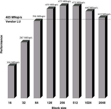
Figure 5.1: Performance of a dense recursive LU factorization with recursive layout of data with varying block sizes compared with vendor LU on the Ultra SPARC II computer for random matrix of size 4096 (the recursive code uses vendor BLAS at a single sub-matrix block level).
Tables 5.1, 5.2, and 5.3 show timing
Table 5.1: Factorization time (t) and forward/backward error estimates after factorization (ξ0, r0) and one iteration of iterative refinement (ξ1, r1) for the test matrices on the SGI Octane computer.
Matrix SuperLU Recursive algorithm name t [s] ξ0 t [s] ξ0 ξ1 r0 r1 af23560 34.57 7×10⁻¹⁴ 34.06 2×10⁻¹⁴ 1×10⁻¹⁵ 2×10⁻⁶ 2×10−7 ex11 85.75 6×10−05 33.47 3×10−07 2×10−07 2×10⁻⁷ 7×10⁻⁷ goodwin 4.48 3×10−08 6.32 5×10−09 3×10⁻¹¹ 7×10⁻⁵ 1×10⁻⁶ jpwh_991 0.18 3×10⁻¹³ 0.16 5×10−08 3×10⁻¹⁵ 3×10+3 5×10⁻⁵ mcfe 0.07 1×10⁻¹³ 0.06 3×10⁻¹³ 3×10⁻¹⁶ 1×10⁻³ 2×10⁻⁵ olafu 18.92 1×10−06 18.83 5×10⁻¹⁰ 9×10⁻¹¹ 1×10⁻⁶ 4×10⁻⁷ orsreg1 0.40 2×10⁻¹⁰ 0.22 5×10−02 2×10−09 9×10+4 1×10⁻¹ psmigr_1 69.44 7×10⁻¹¹ 45.64 4×10−07 8×10⁻¹² 3×10⁻⁴ 4×10⁻⁴ raefsky3 46.26 3×10−09 56.2 8×10⁻¹⁴ 8×10⁻¹⁵ 3×10⁻⁶ 1×10⁻⁷ raefsky4 62.15 3×10−06 64.68 3×10−07 2×10−06 4×10⁻⁶ 6×10⁻⁷ saylr4 0.61 5×10⁻¹¹ 0.52 2×10⁻¹⁰ 3×10⁻¹¹ 5×10⁻⁶ 2×10⁻⁶ sherman3 0.45 5×10⁻¹³ 0.49 2×10⁻¹³ 1×10⁻¹³ 1×10⁻⁶ 7×10⁻⁷ sherman5 0.23 9×10⁻¹⁴ 0.26 2×10⁻¹⁵ 5×10⁻¹⁵ 1×10⁻⁵ 3×10⁻⁶ wang3 73.47 8×10⁻¹⁴ 62.33 1×10⁻¹³ 2×10⁻¹⁵ 1×10⁻⁶ 9×10⁻⁸ ξi = ||xi−x||/||xi|| (relative error at step i) ri = ||Axi−b||/((||A||||xi||+||b||) nє) (backward error at step i)
Table 5.2: Factorization time and forward error estimates for the test matrices for three factorization codes on the Pentium III computer.
Matrix SuperLU UMFPACK 3.0 Recursion name t [s] FERR t [s] FERR t [s] FERR af23560 44.2 5×10⁻¹⁴ 29.3 4×10−04 31.3 2×10−14 ex11 109.7 3×10−05 66.2 2×10−03 55.3 1×10−06 goodwin 6.5 1×10−08 17.8 2×10−02 6.7 5×10−06 jpwh_991 0.2 3×10⁻¹⁵ 0.1 2×10⁻¹² 0.3 3×10⁻¹⁵ mcfe 0.1 1×10⁻¹³ 0.2 2×10⁻¹³ 0.2 9×10⁻¹³ memplus 0.3 2×10⁻¹² 20.1 4×10⁻¹¹ 12.7 7×10⁻¹³ olafu 26.2 1×10−06 19.6 2×10−06 22.1 4×10−09 orsreg_1 0.5 1×10⁻¹³ 0.3 2×10⁻¹² 0.5 2×10⁻¹³ psmigr_1 110.8 8×10⁻¹¹ 242.6 2×10−08 88.6 1×10−05 raefsky3 62.1 1×10−09 52.4 5×10⁻¹⁰ 69.7 4×10⁻¹³ raefsky4 82.5 2×10−06 101.9 5×10+01* 104.3 4×10−06 saylr4 0.9 3×10⁻¹¹ 0.7 2×10−07 1.0 1×10⁻¹¹ sherman3 0.6 6×10⁻¹³ 0.5 2×10⁻¹¹ 0.7 5×10⁻¹³ sherman5 0.3 1×10⁻¹³ 0.3 4×10⁻¹² 0.3 6×10⁻¹⁵ wang3 84.1 2×10⁻¹⁴ 100.1 5×10−08 79.2 2×10⁻¹⁴ t - combined time for symbolic and numerical factorization FERR=||x−x||∞/||x||∞ * the matrix raefsky4 requires for threshold pivoting in UMFPACK to be enabled in order to give a satisfactory forward error
Table 5.3: Total factorization time t, forward error estimate ξ0, and storage requirement η(L+U) for the test matrices for two factorization codes on the Intel Pentium 4 computer.
Matrix SuperLU Recursion name t [s] ξ0 η(L+U) t [s] ξ0 η(L+U) af23560 14.1 5×10⁻¹⁴ 132.2 13.9 1×10⁻¹⁴ 155.7 ex11 36.8 2×10−05 210.2 22.0 1×10−06 159.3 goodwin 2.1 1×10−08 31.3 2.9 1×10−05 41.9 jpwh_991 0.1 2×10⁻¹⁵ 1.4 0.1 2×10⁻¹⁵ 3.4 mcfe 0.01 1×10⁻¹³ 0.9 0.1 9×10⁻¹³ 2.6 memplus 0.1 2×10⁻¹² 5.9 2.7 4×10⁻¹³ 98.7 olafu 8.3 1×10−06 83.9 9.0 7×10−09 104.0 orsreg_1 0.2 1×10⁻¹³ 3.6 0.2 1×10⁻¹³ 5.7 psmigr_1 35.8 7×10⁻¹¹ 64.6 32.4 1×10−05 78.4 raefsky_3 20.0 1×10−09 147.2 27.2 1×10+00 189.5 raefsky_4 26.9 2×10−06 156.2 51.7 4×10−06 241.5 saylr4 0.3 3×10⁻¹¹ 6.0 0.5 1×10⁻¹¹ 11.7 sherman3 0.2 6×10⁻¹³ 5.0 0.4 9×10−01 8.6 sherman5 0.1 1×10⁻¹³ 3.0 0.2 8×10⁻¹⁵ 5.4 wang3 29.3 2×10⁻¹⁴ 116.7 48.9 1×10⁻¹⁴ 246.4
results (the time shown in tables and figures is in seconds unless explicitly stated otherwise) and error estimates for SuperLU Version 2.0 [42, 113] (for sequential machines), UMFPACK Version 3.0 [35, 39] and for the recursive approach. The tables show the total execution time of factorization (including symbolic and numerical phases) and forward error estimates. The matrices used in the tests are selected matrices from the Harwell-Boeing collection [59], and Tim Davis’ [36, 37, 38] matrix collection, which were used to evaluate the performance of SuperLU [42, 113]. Performance of the sparse factorization code heavily depends on the initial ordering of the matrix. Thus, we have selected the best time we could obtain using all the available ordering schemes that come with SuperLU. UMFPACK supports only one kind of ordering (a column oriented version of the Approximate Minimum Degree algorithm [2, 3]), in addition, the code was used with its default values of the tuning parameters and threshold pivoting disabled. For the recursive approach almost all of the matrices were ordered using Reverse Cuthill-McKee ordering [33] except for goodwin and mcfe which were used with their natural ordering. For the recursive approach it is possible to select different block sizes, which yield slightly different execution times. Generally, block size 40 seemed to be optimal; however, for some matrices a better time may be obtained with a different block size (the block sizes tried were between 40 and 120). This coincides with the internal blocking factor of ATLAS [56, 163] that was used as a BLAS implementation. To accommodate CPU and memory hierarchy parameters, ATLAS performs computations on 40 rows or columns at a time and does so in an extremely efficient manner. If the number of rows or columns is not divisible by 40, a so called clean-up code is involved which is slightly less efficient. Consequently, block sizes that are multiples of 40 are preferred when ATLAS is used.
The total factorization time from Tables 5.1, 5.2, and 5.3 favors the recursive approach for some matrices, e.g., ex11, psmigr_1 and wang3, and for others it strongly discourages its use (matrices mcfe, memplus and raefsky4). There are two major reasons for the poor performance of the recursive code on the second group of matrices. First, there is an average density factor which is the ratio of the true nonzero entries of the factored matrix to all the entries in the blocks. It indicates how many artificial non-zeros were introduced by the blocking technique. Whenever this factor drops below 70%, i.e. more than 30% of the factored matrix entries do not come from the L and U factors, the performance of the recursive code will most likely suffer. Even when the density factor is satisfactory, still, the amount of fill-in incurred by the Reverse Cuthill-McKee ordering may substantially exceed that of other orderings. In both cases, i.e. with a low value of the density factor or excessive fill-in, the recursive approach performs too many unnecessary floating point operations and even the high execution rates of the Level 3 BLAS are not able to offset it.
The computed relative and backward errors are similar for all the codes despite the fact that two different approaches to pivoting are used. SuperLU uses threshold pivoting while in UMFPACK and the recursive code there is no pivoting but instead the iterative refinement method is used.
Tables 5.4 and 5.5 show storage requirements and
Table 5.4: Parameters of the test matrices, their storage requirements and floating point operation counts for SuperLU and the recursive algorithm on the SGI Octane computer.
Matrix parameters SuperLU Recursive algorithm Name n η(A) η(L+U) no. flops nB η(L+U) no. flops [MB] [Mflop] [-] [MB] [Mflop] af23560 23560 460598 127.6 4515 50 138.9 5649 ex11 16614 1096948 206.7 14249 50 138.1 10320.5 goodwin 7320 324772 29.9 506 40 41.4 2097.82 jpwh_991 991 6027 1.5 16.1 36 2.3 34.2 mcfe 765 24382 0.7 2.7 34 1.2 11.94 olafu 16146 1015156 80.7 2960 50 90.0 4937 orsreg_1 2205 14133 3.6 43.6 33 3.4 49.05 psmigr_1 3140 543162 64.0 9687 45 73.7 20075.4 raefsky3 21200 1488768 143.1 7752 50 199.7 17618.5 raefsky4 19779 1316789 152.3 10575.6 50 214.3 21593.8 saylr4 3564 22316 5.3 62.3 36 6.3 101.55 sherman3 5005 20033 4.0 46.2 49 5.8 93.95 sherman5 3312 20793 2.3 16.3 40 3.3 44.21 wang3 26064 177168 111.6 9966.5 50 214.9 18140
operation counts for the test matrices. On average, it may be observed that SuperLU and UMFPACK use slightly less memory and perform fewer FP operations. This can be attributed to the minimum degree algorithm and its variations used in SuperLU and UMFPACK which minimize the fill-in and thus the space required to store the factored matrix. The large differences between operation counts come from the fact that the recursive approach stores many more floating point values (most of which are zero). This is not evident from the memory requirements because the storage scheme is very sparing in storage of indices. However, it becomes noticeable in the floating point operation counts which is proportional to the third power of the number of FP values. Nevertheless, the performance in terms of time to solution of the recursive code is still very competitive with SuperLU and UMFPACK due to the judicious use of Level 3 BLAS.
Table 5.5: Parameters of the test matrices and their storage requirements for three factorization codes on the Pentium III computer (for the recursive code the blocking factor nB for the optimal run is also given).
Matrix parameters SuperLU UMFPACK 3.0 Recursion Name n η(A)×10−3 η(L+U) η(L+U) η(L+U) nB [MB] [MB] [MB] af23560 23560 461 132.2 96.6 149.7 120 ex11 16614 1097 210.2 129.2 150.6 80 goodwin 7320 325 31.3 57.0 35.0 40 jpwh_991 991 6 1.4 1.4 2.3 40 mcfe 765 24 0.9 0.7 1.8 40 memplus 17758 126 5.9 112.5 195.7 60 olafu 16146 1015 83.9 63.3 96.1 80 orsreg_1 2205 14 3.6 2.8 3.9 40 psmigr_1 3140 543 64.6 76.2 78.4 100 raefsky3 21200 1489 147.2 150.1 193.9 120 raefsky4 19779 1317 156.2 171.5 234.4 80 saylr4 3564 22 6.0 4.6 7.2 40 sherman3 5005 20 5.0 3.5 7.3 60 sherman5 3312 21 3.0 1.9 3.1 40 wang3 26064 177 116.7 249.7 256.7 120
Finally, Table 5.6 shows comparison of performance of MA41 and the recursive code. The table shows only the numerical factorization time since this is the part of the recursive code that was optimized the most. This is in contrast with MA41 which has been thoroughly tuned in every aspect and in its current form benefits from theoretical and implementation optimizations known in the field of sparse direct methods for symbolic as well as numerical phases of the factorization. As the Table 5.6 shows, MA41 is faster on all of the tested matrices except for mcfe for which the times are the same. Still, the recursive code offers comparable performance levels for matrices af23560, ex11, and olafu. For the rest of the matrices MA41 is a clear winner. Further analysis, that is presented later on, reveals the reason for such extraordinarily good behavior. Namely, the structural symmetry factor has very favorable values for the test matrices and MA41 takes full advantage of it.
Table 5.6: Numerical factorization time for two factorization codes – MA41 and the recursive one – on the Pentium III computer. Symmetry factor was reported by MA41 (100% means structural symmetry).
Matrix parameters Symmetry MA41 Recursion Name n η factor [%] t [s] t [s] af23560 23560 460598 100 12.9 16.2 ex11 16614 1096948 100 29.1 30.9 goodwin 7320 324772 64 1.3 4.5 jpwh_991 991 6027 95 0.05 0.2 mcfe 765 24382 71 0.1 0.1 memplus 17758 126150 100 0.2 4.6 olafu 16146 1015156 100 9.8 10.6 orsreg_1 2205 14133 100 0.1 0.2 psmigr_1 3140 543162 48 39.9 60.1 raefsky3 21200 1488768 100 13.6 36.6 raefsky4 19779 1316789 100 34.5 64.5 saylr4 3564 22316 100 0.2 0.5 sherman3 5005 20033 100 0.2 0.3 sherman5 3312 20793 78 0.1 0.2 wang3 26064 177168 100 39.2 52.6
This section focuses on analysis of performance of the direct solvers presented earlier. In particular, time breakdowns and timings for synthetic data sets are presented to reveal performance characteristics of each code so it becomes possible to draw more insightful conclusions from the previously presented tests as to under what circumstances and in what manner the software packages should be used.
Table 5.7 gives more insight into performance characteristics of UMFPACK. First and foremost, for matrices memplus, olafu, psmigr_1, and raefsky3 the older Fortran version is significantly faster than the new version written in C. It is hard to imagine that the choice of programming language would trigger such a drastic change, especially bearing in mind that for all the other matrices the new version clearly outperforms the older one. More likely explanation is the change in internal algorithms when migrating to C from Fortran. It seems to be supported by more flexible interface in the C version which allows to perform symbolic and numerical phases separately (and possibly reuse the former for structurally identical matrices.)
Table 5.7: Breakdown of time spent in factorization for UMFPACK 3.0 in C and UMFPACK 2.2 in Fortran on the Pentium III computer. (Threshold pivoting was disabled; Fortran version did not allow separation of factorization phases.)
Matrix UMFPACK 3.0 UMFPACK 2.2 name Symbolic Numerical Combined Combined af23560 4.59 23.95 28.54 71.47 ex11 5.35 61.67 67.02 268.54 goodwin 0.89 18.08 18.97 17.19 jpwh_991 0.03 0.11 0.14 0.09 mcfe 0.06 0.1 0.16 0.12 memplus 6.78 11.74 18.52 0.65 olafu 3.04 22.86 25.9 13.85 orsreg_1 0.04 0.31 0.35 0.51 psmigr_1 3.31 247.57 250.88 61.34 raefsky3 1.59 51.17 52.76 45.74 raefsky4 5.10 97.17 102.27 134.04 saylr4 0.07 0.51 0.58 0.88 sherman3 0.06 0.36 0.42 0.71 sherman5 0.08 0.24 0.32 0.63 wang3 0.66 99.36 100.02 331.42
Figures 5.2 and 5.3 show time breakdown
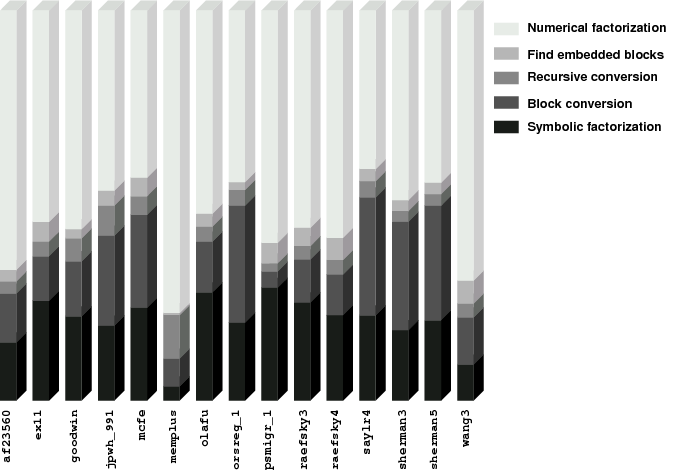
Figure 5.2: Breakdown of time spent in the recursive factorization code with block size 40 on the Pentium III computer.
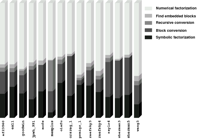
Figure 5.3: Breakdown of time spent in the recursive factorization code with block size 100 on the Pentium III computer.
for the recursive code for block sizes 40 and 100, respectively. The breakdown lists relative time spent in the following phases of the algorithm:
Comparison of Figures 5.2 and 5.3 results in a predictable conclusion that for larger block sizes more FP operations are performed. This may be easily explained by the fact that for larger block sizes more artificial non-zero entries are introduced and therefore there is more data to operate on. The difference is the most conspicuous for the memplus matrix which is more sparse than any other matrix from the tested group. Such an insight offers a guideline for selecting a block size – a balance must be achieved between performance of BLAS – the block size cannot be too small – and excessive number of FP operations – the block size cannot be too large.
Table 5.8 compares numerical factorization times of various block-oriented sparse direct codes (total factorization time is approximately twice as large as the numerical part alone, refer to Figures 5.2 and 5.3 for detailed time breakdown). The table compares two types of codes: the recursive one and a block one operating on symmetric matrix structure (it is a straightforward, loop-based, symmetric-structure code that instead of individual values operates on the same submatrices that the recursive algorithm uses). The former can handle matrices with unsymmetric structure. The latter assumes that the system matrix is structurally symmetric and consequently have the storage and processing is needed to describe and operate on matrix’ structure. If, however, the original matrix is not symmetric in structure then artificial non-zero entries are introduced such that the structure of the matrix becomes symmetric but numerical equivalence is retained. Needless to say, such a naïve procedure might be disastrous in terms of performance for matrices whose structure is far from symmetric and many artificial non-zero entries need to be introduced. The block symmetric code was implemented in C [104, 110] and Python [134] programming languages. A number of interesting observation can be made. On average the recursive code is slightly faster than the iterative code even though the iterative code has roughly twice as little integer arithmetic to perform. This may be attributed to superior memory performance of the recursive code. It also explains why the larger block size yields for quite a few matrices better performance as far as the recursive code is concerned whereas the iterative code almost invariably has worse performance for the larger block size (except for the psmigr_1 matrix which is very dense after fill-in and could use as large block size as possible). The column with timings for the Python code shows how few integer operations are performed in the symmetric code. The Python implementation is comparable to its C counterpart even though it is being interpreted (rather than first compiled and then executed on the CPU). The Python code uses the same optimized BLAS as the other two codes and clearly it is the main prerequisite for performance.
Table 5.8: Numerical factorization times for various block-oriented codes on the Pentium III computer. For the implementation in the Python programming language the time and block size of the fastest run are shown.
Matrix Recursive Symmetric Python symmetric name nB=40 nB=100 nB=40 nB=100 t [s] nB af23560 30.58 17.51 16.2 26.7 17.26 40 ex11 31.51 29.23 30.9 38.7 33.98 40 goodwin 3.81 3.92 4.5 6.5 7.08 40 jpwh_991 0.12 0.16 0.2 0.3 0.21 40 mcfe 0.09 0.13 0.1 0.3 0.13 20 memplus 7.63 3.6 4.6 16.1 5.52 30 olafu 12.86 10.37 10.6 18.1 16.39 40 orsreg_1 0.22 0.23 0.2 0.5 0.26 40 psmigr_1 50.11 52.89 60.1 56.7 57.92 100 raefsky3 42.61 35.91 36.6 44.4 38.41 40 raefsky4 61.45 60.76 64.5 75.1 71.02 40 saylr4 0.39 0.52 0.5 1.2 0.51 40 sherman3 0.35 0.37 0.3 0.6 0.36 40 sherman5 0.15 0.18 0.2 0.4 0.17 40 wang3 70.20 50.80 52.6 61.2 54.85 40
Table 5.9 shows results from experiments on randomly generated skyline matrices. The matrices were generated so they had a changing symmetry factor, i.e. the ratio of all non-zero matrix entries to the number of entries in the minimal numerically equivalent matrix that was symmetric in structure. The ratio is 0% for matrices without any symmetry and 100% for structurally symmetric matrices. The experiments were mainly to show the weakness of the MA41 code – its dependence on matrix’ structural symmetry. While on the tests matrices MA41 performed exceptionally well (see Table 5.6), it is rather slow for highly structurally unsymmetric matrices and becomes more and more competitive as the matrix’ inherent structural symmetry rises. In a sense though, it cannot become competitive enough since the blocked symmetric code, that takes advantage of symmetry just like MA41, is almost consistently better. Surprisingly, SuperLU seems to be well (if not the best) suited for this experimental setting having extremely good overall performance, especially bearing in mind that for SuperLU the total time is reported rather than just numerical factorization time. This turns out to be even more unexpected considering the fact that SuperLU does not use Level 3 BLAS – only Level 2 or lower.
Table 5.9: Numerical (total in the SuperLU case) factorization time for random skyline matrices of order 30000 for various direct codes. Symmetry factor is η(A)/η(A+AT) and is 100% for structurally symmetric matrices.
Symmetry MA41 Unsymmetric Symmetric SuperLU factor [%] t [s] recursion, t [s] blocked, t [s] t [s] 37 22.7 11.6 38.6 9.7 56 36.8 19.9 35.7 19.9 64 54.5 34.5 34.7 29.9 67 136.1 153.2 35.6 39.9
Table 5.10 shows performance results of a reference (unoptimized)
Table 5.10: Performance of the reference and optimized sparse matrix-vector multiplication routines on the Intel Pentium 4 computer.
Matrix Reference Optimized Improvement name [Mflop/s] [Mflop/s] [%] af23560 262.5 295.3 12.5 ex11 279.1 294.2 5.4 gemat11 153.6 307.2 100.0 goodwin 267.6 291.9 9.1 mcfe 240.0 240.0 0.0 memplus 195.5 195.5 0.0 olafu 272.2 287.7 5.7 psmigr_1 285.0 300.9 5.6 raefsky3 268.8 301.7 12.2 raefsky4 269.1 286.7 6.5 saylr4 205.3 205.3 0.0 sherman3 175.3 175.3 0.0 sherman5 191.4 191.4 0.0
implementation of sparse matrix-vector multiplication routine in row-oriented storage format together with a code that utilizes the graph compression technique mentioned earlier (see section 4.7) which allows to take better advantage of standard RISC-oriented optimizations (also described earlier – see section 4.6). The set of the test matrices, although not selected for practical purposes of this study, but rather influenced by external references, turned out to be diversified enough to show both strengths and weakness of the optimization based on graph compression. For matrix gemat11 a 100% performance improvement was possible. While still it might be due to really low performance of the reference code, nevertheless, for this matrix there should be a significant improvement against any other known optimization techniques. Such a good result should be mainly attributed to a high level compression that was possible for this matrix. Unfortunately, the Bi-CGSTAB algorithm does not converge for this matrix and so the gains from the optimization cannot be used to obtain a solution to a linear system (only to detect quicker a breakdown of the solver). On the other hand for quite many (5 in all) matrices there was no visible improvement against reference implementation. For these matrices, no graph compression occurs – the original and compressed graphs are isomorphic. This suggests that the graph compression method should be supplied with other blocking techniques to get at least improvement level. On the positive side, it has to be noted that compression did not slow the multiplication routine. Other than the time that was used to compress the graph, no additional overhead is incurred even if the optimization does not pay off.
Tables 5.11 and 5.12 show performance
Table 5.11: Performance data for the reference (not optimized) Bi-CGSTAB implementation on the Intel Pentium III computer.
Matrix Number of Correct ||Ax−b||∞ tTotal tSDGEMV Perf. tol Name Iterations Digits [-] [s] [s] [Mflop/s] [-] jpwh_991 39 9 2×10−09 0.028 0.016 91 10−09 mat64x32 1739 7 2×10−09 66.5 47.4 91 10−09 memplus 1499 5 1×10⁻¹⁰ 41 26 53 10−09 orsreg_1 545 6 9×10−06 0.95 0.56 69 10−09 psmigr_1 1524 3 1×10−06 95.5 93.1 44 10−12 saylr4 3387 11 6×10⁻¹¹ 12.3 7.9 73 10−09 sherman3 22737 2 4×10−08 100.4 54.0 53 10−14 sherman5 2259 6 2×10−06 7.0 4.2 59 10−09 venkat01 7317 2 1×10−06 1744 1436 33 10−07 wang3 264 8 7×10⁻¹² 10.5 6.4 38 10−09
Table 5.12: Performance data for the optimized Bi-CGSTAB implementation on the Intel Pentium III computer.
Matrix Number of Correct ||Ax−b||∞ tTotal tSDGEMV Perf. tol Name Iterations Digits [-] [s] [s] [Mflop/s] [-] jpwh_991 39 9 5×10−09 0.025 0.014 82 10−09 mat64x32 1765 7 2×10−09 62.3 43.0 38 10−09 memplus 1474 5 2×10⁻¹⁰ 43 27 34 10−09 orsreg_1 484 6 9×10−06 0.73 0.43 79 10−09 psmigr_1 1399 3 1×10−06 83.1 80.9 38 10−12 saylr4 3730 11 6×10⁻¹¹ 11.7 6.8 60 10−09 sherman3 17849 2 4×10−08 78.7 43.1 51 10−14 sherman5 2478 6 2×10−06 7.0 4.4 62 10−09 venkat01 6826 2 1×10−06 1652 1354 36 10−09 wang3 259 8 7×10⁻¹² 9.8 5.9 38 10−09
results on the Pentium III computer for reference (unoptimized) and optimized implementations, respectively, of the Bi-CGSTAB algorithm. Similarly, Tables 5.13 and 5.14 show results for
Table 5.13: Performance data for the reference (not optimized) Bi-CGSTAB implementation on the Intel Pentium 4 computer.
Matrix Number of Correct ||Ax−b||∞ tTotal tSDGEMV tol Name Iterations Digits [-] [s] [s] [-] jpwh_991 39 9 2×10−09 0.006 0.003 10−09 mat64x32 1739 7 2×10−09 10.1 6.0 10−09 memplus 1499 5 1×10⁻¹⁰ 7.17 3.9 10−09 orsreg_1 545 6 9×10−06 0.22 0.13 10−09 psmigr_1 1524 3 1×10−06 11.22 10.7 10−12 saylr4 3387 11 6×10⁻¹¹ 2.46 1.4 10−09 sherman3 22737 2 4×10−08 21.17 10.8 10−14 sherman5 2259 6 2×10−06 1.58 0.9 10−09 venkat01 7317 2 1×10−06 250 186 10−07 wang3 264 8 7×10⁻¹² 1.69 0.9 10−09
Table 5.14: Performance data for the optimized Bi-CGSTAB implementation on the Intel Pentium 4 computer.
Matrix Number of Correct ||Ax−b||∞ tTotal tSDGEMV tol Name Iterations Digits [-] [s] [s] [-] jpwh_991 39 9 5×10−09 0.007 0.003 10−09 mat64x32 1765 7 1×10−09 9.6 5.8 10−09 memplus 1474 5 2×10⁻¹⁰ 6.8 3.7 10−09 orsreg_1 484 6 9×10−06 0.19 0.1 10−09 psmigr_1 1399 3 1×10−06 9.98 9.5 10−12 saylr4 3730 11 6×10⁻¹¹ 2.7 1.6 10−09 sherman3 17849 2 4×10−08 16.6 8.4 10−14 sherman5 2478 6 2×10−06 1.8 1.0 10−09 venkat01 6826 2 1×10−06 222 169 10−09 wang3 259 8 7×10⁻¹² 1.6 0.8 10−09
unoptimized and optimized codes but on the Pentium 4 computer. The tables include timings for matrix mat64x32 which results from circular boundary conditions on a regular grid – it may be regarded as a generic matrix for many model 2D problems that are commonly tackled with iterative methods. To better show how time is distributed between various components of the codes, the time spend in matrix-vector routine (the routine itself is called twice for every iteration – each call is timed and accumulated for all calls) tSDGEMV is also included in the tables. Judging by the number of publications on improvements made to the sparse matrix-vector multiplication routine, it should be natural to conclude that this is where most of the time is spent (barring the use of a preconditioner). The data from the tables to an extent disagree with this assertion – there are matrices (jpwh_991, sherman3, and sherman5) for which only half of the time is spent in the multiplication routine. Thus, it is justifiable to optimize the rest of the code as it was done for the optimized version in Tables 5.12 and 5.14. By using all the optimizations described earlier (see section 4.7), except for graph compression whose influence was shown earlier, it is possible to reduce the time to solution by about 10% on average. An interesting result was obtained for matrix wang3 for which the time is much shorter than for any of the direct methods presented in the preceding sections. The only superiority exhibited by direct methods is accuracy of the solution – twice as many correct digits may be worth spending about six times as much on computations. The rest of the matrices do not pose such a dilemma – any of the direct methods are superior in terms of time and accuracy. The difference is not in order of magnitude, though.
Another comment is due at this point as to why time to solution was used as the performance metric in Tables 5.11, 5.12, 5.13, and 5.14. It might be tempting to report time per iteration and compare it for codes prior and after optimizations. This is especially true bearing in mind that the unoptimized and optimized codes perform different number of iterations (for most of the matrices the optimized code performs less iterations but the difference does not exceed 10%) to achieve the same level of accuracy and trigger the stopping criterion. However, a user-centric view was adopted in reporting the data for the tables. From the user perspective, only the time to obtain a solution (or indication of failure for that matter) and its quality is important. The details of the implementation are of a lesser, if not the least, concern.
Finally, it should be mentioned that Tables 5.11, 5.12, 5.13, and 5.14 do not show results for all the matrices that were used with the direct solvers in the preceding sections, the reason being lack of convergence for the missing matrices. From a theoretical standpoint an iterative method that does not converge should be replaced with a different method. From the user standpoint, however, learning about the failure is as time consuming as delivering a satisfactory solution. Consequently, even an optimized failing code has an advantage over an unoptimized one as the former is able to provide quicker information about failure.
This research completed the set of theoretical results pertaining to the recent algorithmic advances in decompositional techniques of numerical computational linear algebra for dense matrices [67, 95, 157]. In addition, a new formulation of recursive LU factorization algorithm has been proposed and applied in sparse matrix computations. The application was compared with modern software packages. The comparison yielded promising results on a range of modern computing platforms. Aside from competitive studies, thorough performance analysis and time breakdown were presented. Also, mixed-language implementation was tested to give yet greater insight into runtime characteristics of the proposed algorithm.
In the area of iterative methods, time breakdown was presented for the Bi-CGSTAB algorithm while applying it to an interdisciplinary set of sparse matrices. Based on the obtained results, a more holistic approach to optimization of Bi-CGSTAB was shown. The approach incorporates a newly proposed generalization of theoretical advances in symmetric matrix orderings [14] which results in appreciable speed-up of matrix-vector multiplication for certain types of sparse matrices. Additionally, a set of known optimizations was used to improve performance of the remaining part of the Bi-CGSTAB algorithm to provide yet more gains in terms of efficiency and revealing some convergence subtleties which, however, do not diminish the improvements.
The material from this writing could conceivably be extended in ways that might lead to potentially useful results.
The use of recursive matrix layout (or any of its suitable variants [93]) could be incorporated into existing multifrontal or supernodal approaches. This could shed more light on an interesting question as to where the performance comes from in the current implementation, whether it is the algorithm or the data layout.
Extending the existing code so it handles variable size sub-matrices is also an interesting undertaking as it has been successfully used before [90, 141, 142, 143, 144, 160] but without recursive algorithm. Another possibility is to let the recursive algorithm be guided by symbolic data structures like an elimination tree or assembly tree that are naturally created during the symbolic phase of the factorizations. In this context, different recursive tree traversal schemes give wide range of research possibilities. And finally, employing the recursive code as a preconditioner might yield a viable solution in terms of efficiency and numerical terms. A new notion of incompleteness in preconditioning is required, though.
In the context of vector and parallel processing, the basic precept of reduction of memory traffic by the recursive algorithm needs to be revisited and somehow achieve properties that currently favor block-cyclic schemes [131]. Moreover, the use of recursion could be a welcome innovation for factorization codes that need to initially obtain the data from a disk and stage the factored matrix on a disk afterwords.
Certainly, the graph compression technique could use an improvement for matrices without large subsets of vertices with identical adjacency sets – the very matrices that show only moderate, none at all, performance increase. The requirement for the adjacency sets to be identical simplifies and speeds-up the implementation but on the other hand makes its success extensively dependent on matrix structure. Experiments with efficient algorithms for 0-1 matrices [27] could give some insight into possible progress in this areas. Also, naïve algorithms (with exponential computational complexity) for testing similarities (rather than identity) between adjacency sets could be tackled with techniques from the field of Fixed Parameter Tractability [68, 69, 70, 71, 111, 112].
As far as iterative methods are concerned, it would be interesting to see how much slower an iterative solver is for, say, two right-hand sides. If it is comparable, then it might be possible to iterate simultaneously on more than one vector which would increase robustness of any iterative method. Another question is how these simultaneous vectors and their corresponding right-hand sides should be related to yield faster convergence.
The results for block variants of popular iterative solvers do not give enough guidance for possible implementations. The common result on convergence rate for the CG algorithm states that [128, 146]:
| ||x−xi||A≤2||x−x0||A | ⎛ ⎜ ⎜ ⎜ ⎜ ⎝ |
| ⎞ ⎟ ⎟ ⎟ ⎟ ⎠ |
| (6.1) |
for Ax=b linear system with κ being a condition number of A and xi being the iterates. The result (6.1) is proven for each component separately in the case of a block method with multiple right-hand side. Maybe a better monitoring strategy be possible if one or more of the iterated vectors is known from the onset – this would probably require a generalization of equation (6.1).
ℝ set of real numbers A,L,U real matrices: A,L,U∈ℝm× n, A=[aij] 1≤ i≤ m,1≤ j≤ n ||·||p matrix or vector norm: ||x||p=(∑i=1n|xi|p)1/p ||A||p=supx≠0||Ax||p/||x||p ||A||F=(∑i=1m∑j=1n|aij|2)1/2 where: A∈ℝm× n; x∈ℝn m,n∈{1,2,…};1≤ p≤+∞ ||·||A A-norm of a vector (A must be positive definite): ||x||A=√xTAx A∈ℝn× n;x∈ℝn κp(A) p-norm matrix condition number: κp(A)=||A||p ||A−1||p U(A) upper triangular part of the matrix including the diagonal: U(A)=[uij] uij={
aij if i≤ j 0 if i>j L1(A) lower triangular part of the matrix with unitary diagonal: L1(A)=[lij] lij={
0 if i<j 1 if i=j aij if i>j ℙn set of n by n permutation matrices, i.e. identity matrices with rearranged rows η(A) number of (structural) nonzero entries in matrix A n(A) dimension of matrix A mB, nB blocking factors for the first and second matrix dimensions float(x) floating point representation of x є machine floating point precision: є=maxe>0float(1+e)=1 x approximation of x ξ(x,x) relative forward error: ξ(x,x)=(x−x)/x≡FERR(x,x) r(x) scaled residual (backward error) of Ax=b: r(x)=(||Ax−b||)/(||A||||x||nє) logx logarithm of base 2: logx≡log2x (unless stated otherwise) min{…} smallest value O(f(n)) functions of order f(n): O(f(n))= {g∣∃a,b,N∀n>N af(n)≤ g(n)≤ bf(n)}
Vita
Piotr Luszczek was born in Kraków, Poland on October 19, 1974. He graduated from high school in 1989 with the title of Electronics Technician, and received a Master of Science degree in Computer Science in 1999 from the University of Mining and Metallurgy in Kraków, Poland under supervision of Dr. Marian Bubak. His thesis was about parallel runtime support for distributed-memory irregular applications and was a part of joint research effort with the University of Vienna, Austria.
Immediately after completion of the Master’s degree he came to the University of Tennessee Knoxville to pursue the PhD degree under supervision of Prof. Jack Dongarra. While enrolled at the University of Tennessee, he worked on research projects in cooperation with the Hewlett-Packard Company, the Joint Institute for Computational Science and Oak Ridge National Laboratory.
This document was translated from LATEX by HEVEA.