Project 2 — Activation/Inhibition Cellular Automaton
Programming language
You can use whatever programming language you want. In the past,
students have used languages such as C, Java, Python, and Matlab. Warning
about Python: several past students preferred programming in
Python, however, some of them had issues with their programs taking
a long time to run, which is even more of a problem given that you
will need to run quite a few experiments. This project requires that
you implement a 30x30 structure, and it seems that Python has
trouble handling this. So if you choose to use Python, be sure to
start early!
Setting up your code
The CA is two dimensional and the space is 30 units in each
dimension. The most straight-forward way to represent this space is
with a 30x30 array of integers, where each cell contains either 1 or
-1. At the beginning of the program, randomly initialize each cell
to 1 or -1.
You will also want to keep track of the correlation and mutual
information at each possible radius. Probably the easiest way to do
this is to use a 15 element array of doubles for each of the three
measures. The 15 elements account for each of the possible radii
(distances), 0 to 14.
You will also want to keep track of overall entropy and (for 527
students) correlation length (lambda). These variables and the ones
mentioned above should all be global.
In order to help automate the process of collecting data, it will be
helpful to take in all the parameters on the command line. This
includes J1, J2, h, R1,
R2, and possibly an ID number for the
experiment/run that you are executing so that you can properly name
any data files your code will write.
You will also need to average over several runs for each set of
parameters that you test. Four runs for each should be enough. Each
run should have a different random initial state. You may want
additional data structures to keep a running total of individual
runs so that you can compute their averages for each of the
measures.
Displaying the AICA structure
In order to support your analysis and observations of AICA behavior,
it will be very helpful to be able to view the structures generated
by a particular set of parameters. Including several of these images
in your report will enhance your qualitative analysis of the AICAs.
One way to create an image representing an AICA is to use ASCII art.
Simply print the contents of your 30x30 grid to the screen. It the
value of the cell is -1, print a space, and if the cell's value is
1, print a *.
A better way of creating an image depicting the AICA is to write
code to make a .pgm file. For this, you will need a routine to write
data to a file. The top line of the file should read "P2", the
second line should read "30 30", and the third line should read
"255" (no quotes). The remaining lines will contain the pixel values
of the image. Iterate through each cell of your 30x30 grid, and if
the cell's value is 1, print "0 " (black) to the file, and if the
cell's value is -1, print "255 " (white) to the file. Be sure to
include a space after each pixel value, and also write a new line to
the file after each row of the grid.
The problem with the .pgm image is that it is only 30x30 pixels and
therefore too small to see. One way to fix this is to enlarge the
image using an image editing program. Another way is to convert the
.pgm image to .jpg format and display it in a web page where the
height and width can be specified as in the following command
<img src="myimage.jpg" height=100 width=100 border=1>
Another advantage to creating a web page to display the image is
that you can display several images at once, making it easier to
compare images with one another. Using this technique will produce
images like the following examples.


Calculating distance between cells
The distance between two cells is given as the sum of the absolute
difference of the x coordinates and the absolute difference of the y
coordinates, as in the formula
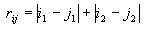
The i and j are the two cells, and the subscripts 1
and 2 denote the x and y coordinates.
In computing the absolute difference of the x coordinates, first
calculate the absolute value of their difference. If this value is
<= 15, then keep it as it is. If this value is > 15, then
subtract it from 30. This accounts for the fact that the space is a
torus where the cell indices are wrapped around on the top and
bottom and the left and right sides. Use this same technique to
compute the absolute difference of the y coordinates. Then just add
these two absolute differences to get the overall distance between
the two cells.
Updating the grid
Before you compute any of the measures, you first need to let the
AICA converge using the following update rule
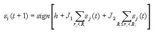
This indicates what state cell i should be in at time step t+1.
It is based on the state of the cell and its neighbors at time step
t. The first term in the brackets is the bias factor h.
The second term gives the effect of nearby cells and the third term
denotes the influence of cells that are farther away.
The cells will be updated one at a time (asynchronously) as opposed
to updating them all at once. So the second cell that gets updated
will depend on the update of the first cell, the third cell to be
updated will depend on the updates of the first and second cell, and
so on. You will want to keep track of which cells have been updated.
A 30x30 array of 0's and 1's corresponding to the grid will work.
The updating process can be implemented with a while loop that runs
until all cells have been updated. First, randomly choose a cell
that has not yet been updated. Then for this randomly chosen cell,
iterate through all the other cells of the grid, computing the
distance between the two cells. If this distance is < R1,
add it to a running total for near cells, and if the distance is
>= R1 and < R2, then add
it to the running total for far away cells. This is how you build
the two summations that are in the update formula. Once you've
iterated through all the other cells, multiply the near sum by J1,
multiply the far sum by J2, then take the sum of
these two products and h to obtain the value in the brackets
of the update formula. If this value is nonnegative, then the new
state of the cell to be updated is 1, otherwise, it is -1.
This updating process is repeated until no cell in the grid has been
changed from a given time step to the next. So there are actually
two nested while loops involved. The inner loop goes until all cells
have been updated, and the outer loop goes until no cell has changed
(i.e. the AICA has stabilized). It should only take a few iterations
for the AICA to stabilize.
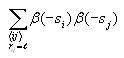
Calculating correlation
The correlation at each possible distance (0 to 14) is calculated
according to the formula
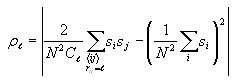
The first term sums over all pairs of distinct cells i and j
and the second term just sums over all cells i. These sums
can be accumulated together through a series of nested for loops.
The outermost for loop iterates through all possible distances l
(0-14). Inside this loop, you will iterate through every cell i
of the grid. For each of these cells i, you will iterate
through all the cells again, these being with subscript j.
You need to be careful that you don't double count cells in your
calculations. You can avoid this by including a conditional on the
indices of the grid cells i and j. If the two row
indices are the same, make sure that the column index of cell j
is greater than the column index for cell i. This will
reject any duplicate cells. After the index check, compute the
distance between cells i and j. If it's the same as
the current distance of the outer for loop, then add the product of
the values of cells i and j to a running total. This
will eventually be the value of the summation in the first term of
the correlation formula. Also within this for loop structure,
accumulate the sum of the values for cell i. After iterating
through all the cells, multiply the summations by the proper
coefficients according to the correlation formula above. Note that N
is 30 and that Cl is 4l, where l
is the current distance (outer for loop variable). Note that if the
distance is 0, then the formula simplifies to
Calculating correlation length (lambda) (427 and 527 students)
Correlation length is a measure of how quickly correlation decreases
with distance, that is, how far away cells must be to have less
effect on each other. Compute this after you have already computed
the correlation for each distance, pl. Then
iterate through the correlations of each distance, and find the one
that is closest to p0/e. The distance
where this happens is the value lambda. It will be given by the
index of the correlation array.
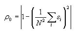
Calculating entropy
First go through each cell in the grid and accumulate the sum of the
converted cell values. To convert the value of a cell, add 1 to it,
then divide by 2. This will be 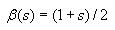 for cell
i.
for cell
i.
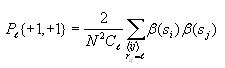
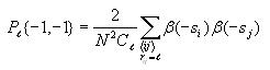
Then compute the probability of state value 1 and the probability of
state value -1 as follows
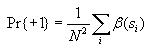
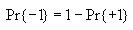
Then use these to compute the overall entropy H(S) as
follows

Note: If Pr{+1} or Pr{-1} is 0, then let their corresponding term in
the formula for H(S) be 0. This will avoid trying to
take the log of 0, which is undefined.
Calculating joint entropy
The joint entropy will be computed for each possible distance l
(0 to 14). Use the same nested for loop structure as in the
computation of correlation and also use the cell index checking
logic for avoiding counting cells twice. Inside all these nested for
loops, compute the following
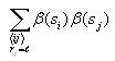
After iterating through all the cells, compute the following

Again, use the technique of avoiding taking the log of 0 as
described above.
Finally, all the pieces can be combined to obtain the joint entropy
for the given distance

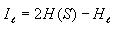
Calculating mutual information
This is very straight-forward. Iterate through each possible
distance l (0 to 14) and compute the mutual information for
each distance as follows
Collecting data
To reduce the amount of tedium, it is a good idea to write the
values of all the measures to a file. If you create a .csv file with
this data, it can be easily opened in Excel where you can feed it
into a graph. The file would contain the values for the parameters J1,
J2, h, R1, and R2,
as well as the values for all the measures you compute, including
correlation, correlation length, overall entropy, and mutual
information. It would contain these values for each of the distances
l. Note that these values would actually be the averages over
the number of runs you do for each set of parameters (probably
around 4 runs each).
Experiments
The objective is to test several different combinations of the five
parameters and investigate their effect on the quantitative measures
and the qualitative behavior of the system. The more parameter
combinations you try, the higher grade you can earn. When I took
this class, I tested a total of 90 different combinations. There are
three top level experiments, each of which will contain their own
set of sub experiments. Following are guidelines for choosing
different sets of parameters.
Experiment 1 (extra credit for 420/427/527): Disable the
inhibition system by setting J2=0 and J1=1.
This means that R2 has no effect on the system,
so the system only depends on R1 and h.
You can try several different values for R1 (eg.
1, 3, 6, 10, 14) and for each of those, try different values of h
starting at 0, and expanding in the positive and negative direction
until you don't see any different behavior or you get an AICA with
all 1's or all -1's.
Experiment 2 (extra credit for 420/427/527):
Disable the activation system by setting J1=0 and
J2=-0.1. This time, vary h, R1,
and R2. For several tests you can fix one
parameter (say R1) and then try several
combinations with R2 and h. Note that R2
should always be greater than R1.
Experiment 3: Enable both activation and inhibition by
setting J1=1 and J2=-0.1.
Again, try different combinations of R1, R2,
and h.
Here is a partial listing of possible experiments to run to give you
the idea of how to vary the parameters. These are all for experiment
3, so J1=1 and J2=-0.1.
1. R1=1, R2=2, h=0
2. R1=1, R2=5, h=-4
3. R1=1, R2=5, h=-2
4. R1=1, R2=5, h=0
5. R1=1, R2=5, h=2
6. R1=1, R2=5, h=4
7. R1=1, R2=9, h=-6
8. R1=1, R2=9, h=-3
9. R1=1, R2=9, h=0
10. R1=1, R2=9, h=3
11. R1=1, R2=9, h=6
12. R1=1, R2=14, h=-6
13. R1=1, R2=14, h=3
14. R1=1, R2=14, h=0
15. R1=1, R2=14, h=3
16. R1=1, R2=14, h=6
17. R1=3, R2=5, h=-1
18. R1=3, R2=5, h=0
19. R1=3, R2=5, h=1
20. R1=3, R2=9, h=-6
21. R1=3, R2=9, h=-3
22. R1=3, R2=9, h=0
23. R1=3, R2=9, h=3
24. R1=3, R2=9, h=6
25. R1=3, R2=14, h=-6
26. R1=3, R2=14, h=-3
27. R1=3, R2=14, h=0
28. R1=3, R2=14, h=3
29. R1=3, R2=14, h=6
30. R1=7, R2=9, h=-1
31. R1=7, R2=9, h=0
32. R1=7, R2=9, h=1
33. R1=7, R2=14, h=-3
34. R1=7, R2=14, h=0
35. R1=7, R2=14, h=3
36. R1=12, R2=14, h=-2
37. R1=12, R2=14, h=0
38. R1=12, R2=14, h=2
Note the systematic way of varying R1, R2,
and h. If you fix all parameters but one, the effect of the
one parameter that does vary will be much more evident. You can draw
conclusions such as "as R1 increases, the
structures get farther apart" or "the system is more chaotic when R1
and R2 are close." Note that these example
conclusions may not describe the actual behavior, they are just for
demonstration purposes.
Note: It would be a good idea to eliminate the cases of all
black and all white from your experiments and/or report since these
cases are uninteresting. You can actually have your code check for
this by seeing if the cells in the grid are all 1s or all -1s.
Expected ranges of values for the quantitative measures:
Here is what you should expect for the range of values for each of
the 3 measures:
Correlation (rho_l): [0, 1]
Joint entropy (H_l): [0, 2]
Mutual information (I_l): [0, 2]
These ranges hold for each of the 3 kinds of experiments.
You should not get any high numbers for these, such as 50 or 80. If
you do, then something is wrong with your code.
You should also never get any negative values for any of
these measures. Of course, if you get NaN for anything, this is also
incorrect. Be sure you are not trying to take the log of 0 or a
negative number.
Generating plots of the quantitative measures
You need to create plots for correlation and mutual information for
most of your parameter combinations. If you wrote your data to a
.csv file, this should be fairly easy to do in Excel. Below is an
example of a graph and a visual representation of the corresponding
AICA. (This graph includes joint entropy, which you do not need to
plot.)
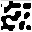
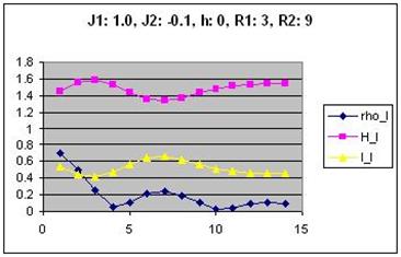
Correlation and mutual information are plotted on the same graph to
facilitate comparison. The values on the x axis are the possible
distances between cells (0 to 14). Part of your analysis might be to
find correlations between the shape of the curves in the graphs and
the structures in the images.
(Revised 2016-02-12)