Wikipedia Links
If you want additional material about hashing, here are Wikipedia Links. As usual with Wikipedia, they tell you far more than you need to know, but you may enjoy the reference material.Overview
Hashing is an important concept in Computer Science. A Hash Table is a data structure that allows you to store and retrieve data very quickly. It is the data structure behind the unordered_set and unordered_map data structures in the C++ Standard Template Library. Although you can use those data structures without knowing what's going on under the hood, this is a computer science class, so you need to learn how hashing and hash tables work.There are three components that are involved with performing storage and retrieval with Hash Tables:
- A hash table. This is a fixed size table that stores data of a given type.
- A hash function: This is a function that converts a piece of data into an integer. Sometimes we call this integer a hash value. The integer should be at least as big as the hash table. When we store a value in a hash table, we compute its hash value with the hash function, take that value modulo the hash table size, and that's where we store/retrieve the data.
- A collision resolution strategy: There are times when two pieces of data have hash values that, when taken modulo the hash table size, yield the same value. That is called a collision. You need to handle collisions. We will detail four collision resolution strategies: Separate chaining, linear probing, quadratic probing, and double hashing.
An example helps to illustrate the basic concept. Let's suppose that our hash table is of size 10, and that we are hashing strings. We'll talk about hash functions later, but let's suppose that we have four strings that we want to store in our hash table: "Luther," "Rosalita", "Binky" and "Dontonio." Let's also suppose that we have a hash function that converts these strings into the following values:
- "Luther" has a hash value of 3249384281.
- "Rosalita" has a hash value of 2627953124.
- "Binky" has a hash value of 216319842.
- "Dontonio" has a hash value of 2797174031.
 |
Similarly, "Rosalita" goes into index 4, and "Binky" into index 2. If we insert them into the hash table, the table looks as follows:
 |
To find a string in the hash table, we calculate its hash value modulo ten, and we look at that index in the hash table. For example, if we want to see if "Luther" is in the hash table, we look in index 1.
Now, suppose we want to look for "Dontonio" in the hash table. Since its hash value is 2797174031, we look in index 1. It's not there. Now suppose we wanted to insert "Dontonio." Well, that's a problem, because "Luther" is already at index one. That is a collision.
I'm not going to fix this problem until later in these lecture notes when we discuss collision resolution strategies. However, it demonstrates why collisions are problems.
Properties of hash tables and hash functions
First, we define the load factor of a hash table to be:(Number of data elements in the hash table) / (Size of the hash table)
That's a pretty intuitively named property. In the hash table pictured above, the load factor is 0.3, because there are three strings in the hash table, and the table size is ten. We can typically quantify how well a hash table is functioning by its load factor.
The selection of a hash function is very important. You want your hash function to have two important properties:
- It should be quick to compute, often constant time, or linear in the size of the data that you are hashing.
- The hash values that it computes should be uniformly distributed from zero to one minus the hash table size. That minimizes collisions.
Interesting Hash Functions for Strings
This page from York University in Canada has some interesting comments about hashing strings. I have programmed up three hash functions for strings -- two from that web page, and one from an article from the journal Communications of the ACM [Pearson90].We start with the most obvious hash function for strings -- add up the ASCII values of the characters. I'm going to call this hash function "BAD". I have this programmed in src/badhash.cpp:
/* This program hashes strings that it reads from standard input
   by simply adding their ascii values.  This is an easy hash function
   to write, but it performs very badly, because the hash values that
   it produces are very similar to each other.  Think about it:
   "abc", "acb", "bac", "bca", "cab" and "cba" all hash to the same value! */

#include <iostream>
#include <string>
using namespace std;

unsigned int bad_hash(const string &s)
{
  size_t i;
  unsigned int h;

  h = 0;

  for (i = 0; i < s.size(); i++) {
    h += s[i];
  }
  return h;
}

int main()
{
  string s;
  unsigned int h;

  while (getline(cin, s)) {
    h = bad_hash(s);
    cout << h << endl;
  }
  return 0;
}
|
Why the unsigned int? The reason is that I want to allow my hash values to go into any 32-bit integer, and I don't want negative numbers. To do that, I specify that the integer be unsigned. Knowing that the ASCII value of 'A' is 65 and that the ASCII value of 'a' is 97, we can verify that the hash function works as advertised:
UNIX> badhash
A
65
a
97
Aa
162
<CNTL-D>
UNIX>
The program in src/djbhash.cpp programs the "DJB" hash function from the York University page:
unsigned int djb_hash(const string &s)
{
  size_t i;
  unsigned int h;

  h = 5381;

  for (i = 0; i < s.size(); i++) {
    h = (h << 5) + h + s[i];
  }
  return h;
}
|
Although the web page says that this is equivalent to:
| hi = 33hi-1 ^ s[i] |
where the carat operator is bitwise exclusive-or, that is not what is implemented. Instead, we take hi-1 and "bit-shift" it, five places to the left. That is equivalent to multiplying by 32, which is 25. However if any of the leftmost 5 bits of the number are set, they are "shifted away" -- they go away. We then add hi-1 -- that is how the author performs multiplication by 33. Finally, we add s[i] rather than performing the bitwise exclusive-or. I don't know why -- I'm just copying code from the web page.
We can double-check ourselves though:
UNIX> bin/djbhash
a
177670                                  5381 * 33 + 97 = 177670
aA
5863175                               177670 * 33 + 65 = 5863175
aAA
193484840                            5863175 * 33 + 65 = 193484840
aAAA
2090032489
<CNTL-D>
UNIX>
That last number takes a little work to verify. First, let's look at 193484840 in hexadecimal (you can do this in C++, but the scripting language awk supports printf, so it's easier):
UNIX> echo 193484840 | awk '{ printf "0x%08x\n", $1 }'
0x0b885828
UNIX>
As mentioned in previous lectures, hexadecimal allows you to look at bytes -- every two
hex digits is a byte: 0b, 88, 58, 28. Breaking this down further, each hexadecimal digit
represents four bits, so the number is:
0000 1011 1000 1000 0101 1000 0010 1000 |
Performing the left bit-shift by 5 turns this number into:
0111 0001 0000 1011 0000 0101 0000 0000 |
I've tried to use the blue color to help you -- those are the original bits that remain after the bit-shift. This is 0x710b0500 in hex, which is 1896547584 in decimal (see your lab for how to do that conversion). And finally, 1896547584 + 193484840 + 65 = 2090032489. We've verified that the function works!!
One last hash function comes from [Pearson10]. We'll call it ACM. It uses a permutation table to calculate the hashes: src/acmhash.cpp:
/* This hash function comes from an Article in Communications of the ACM
   in June, 1990.  It uses a permutation table to calculate the hash of
   the next byte, from the hash of the previous byte run through this
   permutation table.  I perform this operation on four different
   bytes, and then calculate a final integer from the bytes. */

#include <iostream>
#include <string>
using namespace std;

static unsigned char perm_table[256] = {
  1, 87, 49, 12, 176, 178, 102, 166, 121, 193, 6, 84, 249, 230, 44, 163,
  14, 197, 213, 181, 161, 85, 218, 80, 64, 239, 24, 226, 236, 142, 38, 200,
  110, 177, 104, 103, 141, 253, 255, 50, 77, 101, 81, 18, 45, 96, 31, 222,
  25, 107, 190, 70, 86, 237, 240, 34, 72, 242, 20, 214, 244, 227, 149, 235,
  97, 234, 57, 22, 60, 250, 82, 175, 208, 5, 127, 199, 111, 62, 135, 248,
  174, 169, 211, 58, 66, 154, 106, 195, 245, 171, 17, 187, 182, 179, 0, 243,
  132, 56, 148, 75, 128, 133, 158, 100, 130, 126, 91, 13, 153, 246, 216, 219,
  119, 68, 223, 78, 83, 88, 201, 99, 122, 11, 92, 32, 136, 114, 52, 10,
  138, 30, 48, 183, 156, 35, 61, 26, 143, 74, 251, 94, 129, 162, 63, 152,
  170, 7, 115, 167, 241, 206, 3, 150, 55, 59, 151, 220, 90, 53, 23, 131,
  125, 173, 15, 238, 79, 95, 89, 16, 105, 137, 225, 224, 217, 160, 37, 123,
  118, 73, 2, 157, 46, 116, 9, 145, 134, 228, 207, 212, 202, 215, 69, 229,
  27, 188, 67, 124, 168, 252, 42, 4, 29, 108, 21, 247, 19, 205, 39, 203,
  233, 40, 186, 147, 198, 192, 155, 33, 164, 191, 98, 204, 165, 180, 117, 76,
  140, 36, 210, 172, 41, 54, 159, 8, 185, 232, 113, 196, 231, 47, 146, 120,
  51, 65, 28, 144, 254, 221, 93, 189, 194, 139, 112, 43, 71, 109, 184, 209};

unsigned int acm_hash(const string &s)
{
  size_t i, j;
  unsigned int h;
  unsigned char byte_hash[4];     /* I'm using a C-style array rather than a vector. */

  /* You keep track of the four bytes in byte_hash, and
     at character j, you operate on byte_hash[j%4]. */

  for (j = 0; j < 4; j++) byte_hash[j] = 0;
  j = 0;
  for (i = 0; i < s.size(); i++) {
    byte_hash[j] = perm_table[byte_hash[j]] ^ s[i];
    j++;
    if (j == 4) j = 0;
  }

  /* At the end, you build the 32-bit hash value from the four bytes. */

  h = 0;
  for (j = 0; j < 4; j++) h = (h << 8) | byte_hash[j];
  return h;
}
|
Now, I know this is a little confusing, but such is life. The permutation table contains a permutation of the numbers between 0 and 255. We then calculate the hashes as follows:
Otherwise: hi =
perm_table[hi-4] ^ s[i]
Again, the carat is the bitwise exclusive-or operator. After calculating all the hi, we only consider the last four. These are held in the array byte_hash. Specifically, byte_hash[0] holds whichever of the last four hi has (i%4) = 0. byte_hash[0] holds whichever of the last four hi has (i%4) = 1, and so on. We then construct h so that byte_hash[0] is the first byte, byte_hash[1] is the second byte, and so on.
Let's walk through some examples:
UNIX> bin/acmhash
a
1610612736
abca
1617125984
abcaa
3848495712
<CNTL-D>
UNIX>
To help you with these examples, let me turn the permutation table in the code above to one that is easier to navigate by hand. It presents the table as 16 rows of 16 hex digits:
Permutation                   Second hex digit
   Table
                 0  1  2  3  4  5  6  7  8  9  a  b  c  d  e  f
                -- -- -- -- -- -- -- -- -- -- -- -- -- -- -- --
             0  01 57 31 0c b0 b2 66 a6 79 c1 06 54 f9 e6 2c a3
             1  0e c5 d5 b5 a1 55 da 50 40 ef 18 e2 ec 8e 26 c8
             2  6e b1 68 67 8d fd ff 32 4d 65 51 12 2d 60 1f de
    First    3  19 6b be 46 56 ed f0 22 48 f2 14 d6 f4 e3 95 eb
     hex     4  61 ea 39 16 3c fa 52 af d0 05 7f c7 6f 3e 87 f8
    digit    5  ae a9 d3 3a 42 9a 6a c3 f5 ab 11 bb b6 b3 00 f3
             6  84 38 94 4b 80 85 9e 64 82 7e 5b 0d 99 f6 d8 db
             7  77 44 df 4e 53 58 c9 63 7a 0b 5c 20 88 72 34 0a
             8  8a 1e 30 b7 9c 23 3d 1a 8f 4a fb 5e 81 a2 3f 98
             9  aa 07 73 a7 f1 ce 03 96 37 3b 97 dc 5a 35 17 83
             a  7d ad 0f ee 4f 5f 59 10 69 89 e1 e0 d9 a0 25 7b
             b  76 49 02 9d 2e 74 09 91 86 e4 cf d4 ca d7 45 e5
             c  1b bc 43 7c a8 fc 2a 04 1d 6c 15 f7 13 cd 27 cb
             d  e9 28 ba 93 c6 c0 9b 21 a4 bf 62 cc a5 b4 75 4c
             e  8c 24 d2 ac 29 36 9f 08 b9 e8 71 c4 e7 2f 92 78
             f  33 41 1c 90 fe dd 5d bd c2 8b 70 2b 47 6d b8 d1
</pre>
|
In the first example, recall that 'a' is 97, which is 0x61 in hex. Let's use that fact to calculate h0 from the equation and table above:
| h0 | = | perm_table[h-4] ^ 0x61 |
| = | perm_table[0x00] ^ 0x61 | |
| = | 0x01 ^ 0x61 | |
| = | 0x60 |
Since the string is only one character long, h1, h2 and h3 are all equal to zero. Therefore, h is equal to 0x60000000. Check it out:
UNIX> echo 1610612736 | awk '{ printf "0x%08x\n", $1 }'
0x60000000
UNIX>
When we try "abca", we have the following ('b' is 0x62 and 'c' is 0x63):
| h0 | = | 0x60. # From above. |
| h1 | = | 0x63. # This is equal to 0x01 ^ 0x62 = 0x63. |
| h2 | = | 0x62. # This is equal to 0x01 ^ 0x63 = 0x62. |
| h3 | = | 0x60. # It is calculated the same as h0 |
Therefore, the hash value should be:
    (h_0 = 0x60) << 24 |
    (h_1 = 0x63) << 16 |
    (h_2 = 0x62) <<  8 |
    (h_3 = 0x60) <<  0 ) =  0x60636260
Let's confirm:
UNIX> echo acba | bin/acmhash
1617060704
UNIX> echo acba | bin/acmhash | awk '{ printf "0x%08x\n", $1 }'
0x60626360
UNIX>
And finally, when we do "abcaa", we know that
h0,
h1,
h2 and
h3 are equal to 0x60, 0x63, 0x62 and 0x60 respectively. Let's calculate
h4 from
h0, the character 'a' (which is 0x61), and the permutation table:
| h4 | = | perm_table[h0] ^ 0x61 |
| = | perm_table[0x60] ^ 0x61 | |
| = | 0x84 ^ 0x61 | |
| = | (1000 0100) ^ (0110 0001) | |
| = | (1110 0101) | |
| = | 0xe5 |
Thus, h is equal to 0xe5636260:
UNIX> echo abcaa | bin/acmhash
3848495712
UNIX> echo abcaa | bin/acmhash | awk '{ printf "0x%08x\n", $1 }'
0xe5636260
UNIX>
Yay!!
I know that was detailed and probably difficult for you. To practice, try: handouts/in_class_1.html in class.
Evaluating how good those three hash functions are
Ok -- now, the claim is that DJB and ACM are good, and BAD is not. Let's do a simple example. The file files/names_100000.txt has 100,000 randomly generated names:UNIX> wc files/names_100000.txt 100000 216288 1599207 files/names_100000.txt UNIX> head files/names_100000.txt Charlie Muffin Alexandra Map Sophia Compensatory Jack Havoc PhD Joseph Tawny Kaylee Torture Addison Oppressor Sophie Tercel Caleb Troglodyte Victoria Garish UNIX>Let's suppose we wanted to create a hash table with these names, and that the hash table's load factor is 0.5. Thus, we'll make the table size 200,000. We can see the hash values generated by piping badhash, djbhash and acmhash to awk, which will print the hash value mod 200,000:
UNIX> head files/names_100000.txt | bin/badhash | awk '{ print $1%200000 }'
1341
1230
1928
1190
1180
1392
1711
1255
1572
1471
UNIX> head files/names_100000.txt | bin/djbhash | awk '{ print $1%200000 }'
121954
19475
49837
65483
86881
97205
141524
12204
127017
54052
UNIX> head files/names_100000.txt | bin/acmhash | awk '{ print $1%200000 }'
10430
173738
65289
133744
46463
21690
76893
59060
133035
185216
UNIX>
You should see a red flag with BAD. All of those numbers are between 1000 and 2000.
That's because the ASCII values of characters are between 67 and 127 (roughly), and if a name
has 15 characters, that will give you hash values between 67*15 and 127*15. In other words,
roughly between 1000 and 2000. That's not very good. The others look more random.
To evaluate even more, let's calculate all 100,000 hash values, pipe it through awk to print the numbers mod 200,000 and then pipe that through sort -un. This sorts the values numerically, stripping out duplicates. If we pipe that to wc, we can see how many distinct values are produced. The higher that number, the fewer collisions there are:
UNIX> cat files/names_100000.txt | bin/badhash | awk '{ print $1%200000 }' | sort -un | wc
    2305    2305   11106
UNIX> cat files/names_100000.txt | bin/djbhash | awk '{ print $1%200000 }' | sort -un | wc
   78605   78605  506578
UNIX> cat files/names_100000.txt | bin/acmhash | awk '{ print $1%200000 }' | sort -un | wc
   78610   78610  506934
UNIX>
You can see how BAD produces just 2305 distinct hash values, while the others produce roughly
78600. They do a much better job of reducing collisions: only 25% of the hash values collide.
Collision Resolution Strategy Number One: Separate Chaining
Separate Chaining is really simple. Instead of having each element of the hash table store a piece of data, each element stores a vector of data. When you insert something new into the table, you simply call push_back() on the vector at the proper index. When you search for a piece of data, you have to search through the vector.The nice thing about separate chaining is that it does not place limitations on the load factor. It should be pretty clear that if the load factor of a hash table with separate chaining is x, then the average size of each vector is x. That means that to find a piece of data in a hash table, the performance is going to linearly dependent on x. We'll demonstrate that below.
The code in src/cc_hacker.cpp programs up a simple hash table with separate chaining. It stores names and credit card numbers in the hash table. As command line arguments, it accepts a hash table size and a file of credit card numbers/names as in files/cc_names_10.txt:
5034036940778753 Samantha Bustle 9614647402933149 Sydney Macaque 9520044178288547 Eli Boone 4591437720049815 Lillian Handiwork 9464976002919633 Carson Shipmen 1263239861455040 Joshua Lucid IV 1750256670725811 Aaron Flaunt 8988852954721062 Brooklyn Samantha Hoofmark 8293347969318340 Avery Parsifal 1579529982933479 Alyssa Kissing |
For each line, it creates a Person instance, calculates a hash of the name using DJB and then inserts the name into the hash table. Since we're using separate chaining, the hash table is a table of Person vectors. To insert a Person, we calculate the hash of the name, take it modulo the table size and call push_back() on the vector that is there.
After reading the table, we read names on standard input, and look them up in the table.
Here's an example:
UNIX> djbhash
Sydney Macaque
1929449534
Eli Boone
3852330034
Samantha Bustle
2419233313
Jim Plank
2620064763
<CNTL-D>
UNIX> bin/cc_hacker 10 files/cc_names_10.txt
Enter a name> Sydney Macaque
Found it: Table entry 4: Sydney Macaque 9614647402933149
Enter a name> Eli Boone
Found it: Table entry 4: Eli Boone 9520044178288547
Enter a name> Samantha Bustle
Found it: Table entry 3: Samantha Bustle 5034036940778753
Enter a name> Jim Plank
Not found.  Table entry 3
Enter a name> <CNTL-C>
UNIX>
Both "Eli Boone" and "Sydney Macaque" have hash values that equal 4 modulo 10. Therefore, they are in the same "chain". "Samantha Bustle" and "Jim Plank" both have hash values of 3 -- "Samantha Bustle" is in the hash table, and "Jim Plank" is not.
As mentioned above, the average number of entries in each "chain" is equal to the load factor. Therefore, the performance of lookup will be proportional to the load factor.
To demonstrate this, the file files/cc_names_100K.txt has 100,000 random names/credit cards, and files/cc_just_names_100K.txt has just the names, in a different order.
As we increase the table size, the program runs faster: (Redirecting standard output to /dev/null simply says to not print standard output).
UNIX> time bin/cc_hacker 10 files/cc_names_100K.txt < files/cc_just_names_100K.txt > /dev/null
18.283u 0.234s 0:18.51 100.0%	0+0k 0+0io 0pf+0w
UNIX> time bin/cc_hacker 100 files/cc_names_100K.txt < files/cc_just_names_100K.txt > /dev/null
2.294u 0.098s 0:02.39 99.5%	0+0k 0+0io 0pf+0w
UNIX> time bin/cc_hacker 1000 files/cc_names_100K.txt < files/cc_just_names_100K.txt > /dev/null
0.545u 0.072s 0:00.61 100.0%	0+0k 0+1io 0pf+0w
UNIX> time bin/cc_hacker 10000 files/cc_names_100K.txt < files/cc_just_names_100K.txt > /dev/null
0.385u 0.070s 0:00.45 100.0%	0+0k 0+0io 0pf+0w
UNIX>
If we instead try to look up 100,000 names that are not in the table, will it run faster or slower? You tell me.
Collision Resolution Strategies 2-4: Open Addressing
The remaining three collision resolution strategies fall under the heading of open addressing. In these strategies, each element of the hash table holds exactly one piece of data. For that reason, you cannot have a load factor greater than one. In all of these, the ideal load factor is around 0.5. Is that wasteful? Probably not too much, especially if the size of your data is large (the table will store pointers, so the table itself won't consume much room).You may think that open addressing is stupid -- computers have tons of memory these days, so separate chaining should work easily. However, suppose you have to work in constrained environments (e.g. embedded processors, Raspberry Pi, IOT devices) with much tighter memory requirements. Then, being able to preallocate your hash table might be very important.
The remainder of these lecture notes are without computer code, because I want to give you the joy of programming these collision resolution strategies yourself!
With open addressing, you will generate a sequence of hash values for a given key until you find a value that corresponds to a free slot in the hash table. To be precise, you will generate a sequence of hash values, h0, h1, h2, ..., and you look at each in the hash table until you find the value (when you are doing look up), or until you find an empty hash table entry (when you are inserting, or when you are looking up a value that is not there). The various hi are defined as:
H() is the hash function, and F() is a function that defines how to resolve collisions. It is usually convenient to make sure that F(0, key) equals zero, and it is necessary for F(i, key) not to equal zero when i doesn't equal zero.
Linear Probing
With linear probing, F(i, key) = i. Thus, you check consecutive hash sequences starting with H(key) until you find an empty one. Here's an example. Suppose our hash table size is ten, and we want to insert the keys "Luther", "Rosalita", "Binky", "Dontonio", and "Frenchy", using the DJB hash function. Let's first look at their hash values:UNIX> bin/djbhash Luther 3249384281 Rosalita 2627953124 Binky 216319842 Dontonio 2797174031 Frenchy 561643892 <CNTL-D> UNIX>These are the same hash values as in the beginning of these notes, so when we insert "Luther", "Rosalita" and "Binky", they will hash to indices 1, 4 and 2 respectively, so there are no collisions. Here's the hash table:
|
Dontonio hashes to 1, so we have a collision. Formally:
| h0 | = | (2797174031 + 0) % 10 = 1 |
| h1 | = | (2797174031 + 1) % 10 = 2 |
| h2 | = | (2797174031 + 2) % 10 = 3 |
Therefore, we insert "Dontonio" into index 3:
 |
Similarly, "Frenchy" hashes to 2, so it collides and ends up in index 5:
 |
If we try to find the key "Baby-Daisy", we first find its hash value using djbhash: 2768631242. We'll have to check indices 2, 3, 4 and 5 before we find that index 6 is empty and we can conclude that "Baby-Daisy" is not in the table.
One problem with linear probing is that you end up with clusters of filled hash table entries, which can be bad for performance. That fact motivates the next two collision resolution strategies.
Quadratic Probing
As the wikipedia page says, with quadratic probing, F(i, key) = c1i + c2i2. That's pretty general. Typically, when you learn quadratic probing, F(i, key) = i2. We'll go with that in these lecture notes, and if I ask for a definition of quadratic probing, please just say that F(i, key) = i2.We'll use the same example -- "Luther", "Rosalita" and "Binky" are in the hash table and we want to insert "Dontonio".
|
Since there is a collision, we test values of hi until we find one that's not in the table:
| h0 | = | (2797174031 + 02) % 10 = 1 |
| h1 | = | (2797174031 + 12) % 10 = 2 |
| h2 | = | (2797174031 + 22) % 10 = 5 |
Thus, "Dontonio" goes into index 5:
 |
Now when we insert "Frenchy", it collides at h0 = 2, but not at h1 = 3:
 |
If we try to find "Baby-Daisy", we'll check indices 2, 3 and 6 to determine that she is not in the table.
Quadratic Probing can have an issue that all hash table entries are not checked by the various hi. For example, suppose we've inserted "Luther" (3249384281), "Rosalita" (2627953124), "Princess" (2493584940), "Thor" (2089609346), "Waluigi" (385020695) and "Dave" (2089026949) into the table:
 |
Suppose we want to now insert "Peach", which has has a hash value of 232764550. We go through the following sequences of hi:
| h0 | = | (232764550 + 02) % 10 = 0 |
| h1 | = | (232764550 + 12) % 10 = 1 |
| h2 | = | (232764550 + 22) % 10 = 4 |
| h3 | = | (232764550 + 32) % 10 = 9 |
| h4 | = | (232764550 + 42) % 10 = 6 |
| h5 | = | (232764550 + 52) % 10 = 5 |
| h6 | = | (232764550 + 62) % 10 = 6 |
| h7 | = | (232764550 + 72) % 10 = 9 |
| h8 | = | (232764550 + 82) % 10 = 4 |
| h9 | = | (232764550 + 92) % 10 = 1 |
| h10 | = | (232764550 + 102) % 10 = 0 |
| h11 | = | (232764550 + 112) % 10 = 1 |
| ... | ||
That's a problem, as we can't put "Peach" into the table. You need to do a little math to help ensure that hi covers all possible values. Having the table size be prime helps, as would different settings of c1 and c2 in the more general version of quadratic probing.
Double Hashing
With double-hashing, you have a separate hash function, H2. Then, F(i, key) = H2(key)*i. For this to work, H2(key) modulo the table size cannot equal zero.Let's try an example -- let's have H2 be equal to acmhash modulo the table size, and if that value is equal to 0, then set it to one. We'll start with "Luther", "Rosalita" and "Binky" in the table:
|
Again, we want to insert "Dontonio", whose hash value is 2797174031. Since that collides, we need to calculate H2("Dontonio"), which equals 2511778359%10 = 9. Thus h1 = (2797174031+9)%10 = 0, and we can put "Dontonio" into index zero:
 |
Next comes "Frenchy", whose hash value is 561643892. That collides, so we calculate H2("Frenchy"), which equals 3425106287%10 = 7. Thus h1 = (561643892+7)%10 = 9, and we can put "Frenchy" into index nine:
 |
Suppose we want to find "Baby-Daisy". Her hash value is 2768631242, which collides with "Binky". H2("Baby-Daisy") is equal to 2774673939%10=9. Therefore, we'll check hash locations 1, 0, 9 and 8 before seeing that she is not in the hash table.
Finally, as with quadratic probing, you need to be careful with double hashing. Suppose I try to insert "Ryan" into the hash table. The DJB hash value is 2089555519 and the ACM hash value is 1400397935. Do you see why that's problematic:
| h0 | = | (2089555519 + 0*5) % 10 = 9 |
| h1 | = | (2089555519 + 1*5) % 10 = 4 |
| h2 | = | (2089555519 + 2*5) % 10 = 9 |
| h3 | = | (2089555519 + 3*5) % 10 = 4 |
| ... | ||
You can fix the problem in a few ways. The easiest, as with quadratic probing, is to make sure that the table size is a prime number. There are other fixes, but I won't go into them (maybe in class).
Deletion
You should be able to see pretty clearly that you can't delete entries simply when you are using open addressing. We will not discuss that further in this class, but you should be aware of it.At this point, we may go over handouts/in_class_2.html in class. If we don't, then use it as study material.
Load Factors, Collision Resolution and Performance
In your lab, you'll be writing a program that accepts commands to insert and find keys in a hash table. You'll be implementing linear probing and double-hashing as collision resolution strategies. Let's not worry about the details of the hash functions yet -- you'll deal with that with your lab. However, I want to demonstrate how double-hashing is superior to linear probing, but that you want the table size to be a prime number. Your lab program, bin/hash_tester (this is in the lab directory, not here), is called as follows:UNIX> bin/hash_tester usage: hash_tester table-size fxn(Last7|XOR) collision(Linear|Double) [prompt] UNIX> echo '?' | bin/hash_tester 417 Last7 Linear A key val Add the given key/val pair to the hash table. F key Find the given key in the hash table. P Print the hash table. TP Print the total probes for finding all keys. Q Quit. ? Print comands. UNIX>Again, don't worry about the hash function -- we'll call it with "Last7". The keys accepted by this program are any stream of hex digits (so that it can work on things like MD5 and SHA1 hashes). We are going to evaluate this program on the file files/Pictures-SHA1.txt, which contains SHA-1 hashes of 417 of my pictures. In the file, each line starts with "A", so that we can use it as input to bin/hash_tester:
UNIX> head -n 3 files/Pictures-SHA1.txt
A ec9d7382dede0a361ceed9f5933ab682a46b9981 Data/019950.JPG
A fdc4f5f5519546c84d77c15b4df2a33beb1129af Data/019951.JPG
A c6b6843d938f8d338d1e59308ced316d6941c1a0 Data/019952.JPG
UNIX>
Let's see how many probes it takes when we insert it into a hash table with 417 entries. In other words, the load factor is 1.0:
UNIX> ( cat files/Pictures-SHA1.txt ; echo "TP" ) | bin/hash_tester 417 Last7 Linear
4896
UNIX>
Man, that's terrible! Of course, that's what the theory says. Let's double the size of the hash table, as theory recommends:
UNIX> ( cat files/Pictures-SHA1.txt ; echo "TP" ) | bin/hash_tester 834 Last7 Linear
211
UNIX>
That's much better. Let's try double-hashing, with a load factor of 1 (your program will implement two hash functions, called "Last7" and "XOR" -- we use "XOR" as the second hash function in double-hashing):
UNIX> ( cat files/Pictures-SHA1.txt ; echo "TP" ) | bin/hash_tester 417 Last7 Double
A 0722c16fb69be89210669336d65a76132d2cc8d2 Modified/020103.JPG
Cannot insert key
A c07e8c9463217238bce4183a37bf4479b36d3a38 Originals/020099.JPG
Cannot insert key
1402
UNIX>
Well, it's better than linear probing, but 1402 probes is still pretty bad. Moreover, two entries could not be put into the hash table at all! Why? Well, 417 is not a prime number. It is equal to 3 * 139. So if there is a collision, and the second hash value is 139, then you only have three places to look before giving up. If we try 419 (the smallest prime number ≥ 417), there are still a lot of probes, but at least you can get everything into the hash table:
UNIX> ( cat files/Pictures-SHA1.txt ; echo "TP" ) | bin/hash_tester 419 Last7 Double
1641
UNIX>
Take a look at the shell script in the file scripts/evaluate.sh (again this is in the lab directory, not this directory):
#!/bin/sh

for collision in Linear Double ; do
  for table_size in \
      419 421 431 433 439 443 449 457 461 463 467 479 487 491 499 \
      503 509 521 523 541 547 557 563 569 571 577 587 593 599 \
      601 607 613 617 619 631 641 643 647 653 659 661 673 677 683 691 \
      701 709 719 727 733 739 743 751 757 761 769 773 787 797 \
      809 811 821 823 827 829 839 ; do
    echo $collision $table_size \
    `( cat files/Pictures-SHA1.txt ; echo TP ) | bin/hash_tester $table_size Last7 $collision`
 done
done
|
This tests linear probing and double-hashing on every prime table size from 419 (roughly a load factor of one) to 839 (roughly a factor of two). Running it gives us a line for each test, as follows:
UNIX> sh scripts/evaluate.sh | head -n 3
Linear 419 4808
Linear 421 8588
Linear 431 1722
UNIX> sh scripts/evaluate.sh | grep Double | head -n 3
Double 419 1641
Double 421 1466
Double 431 1073
UNIX>
You can take the output of this and put it into your favorite graphing package (I use jgraph, because it works really well with a Unix-based workflow), to see how these collision resolution techniques fare:
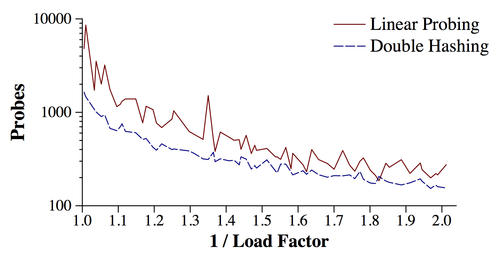 |
As you can see, the graph lines are not smooth, but that is because this is just one set of examples, and the exact number of probes can depend on the luck of the draw. We could smooth this by running lots of different examples, but I'm not going to do that. (Were I to write a paper on this, I'd have to do that so that my graphs are more cogent.) However, I think that the graph pretty clearly allows you to draw the conclusion that Quadratic Probing is superior to Linear Probing on this data.
Cryptographic Hash Functions and the Avalanche Effect
There are several well-known algorithms that compute hash functions of arbitrarily-sized data. One example is the MD5 function that produces a 128-bit hash function from any sized data. Another example is SHA-1, which produces a 160-bit hash. Both functions attempt to generate uniformly distributed hashes from arbitrary data that are secure, in that you can't get any information about the data from the hash. I won't go into a discussion beyond that, except that SHA-1 does a better job, but is more computationally expensive. For our purposes, we will assume that the functions produce hashes from data that look like random streams of bits.The openssl command generates hashes from files using either technique. For example:
UNIX> cat files/input-1.txt
Rosalita, jump a little lighter.
Senorita come sit by my fire.
UNIX> cat files/input-2.txt
Sosalita, jump a little lighter.
Senorita come sit by my fire.
UNIX> openssl md5 files/input-1.txt files/input-2.txt
MD5(files/input-1.txt)= b9937df3fefbe66d8fcdda363730bf14
MD5(files/input-2.txt)= 3a752ef1b9bfd1db6ba6a701b6772065
UNIX> openssl sha1 files/input-1.txt files/input-2.txt
SHA1(files/input-1.txt)= 9a2c3d93445fa844094eb213a17fc5996895c925
SHA1(files/input-2.txt)= 8886b6ef4671093b15c2dba387c3eb169e9db5d2
UNIX>
The representation of the hashes is a long stream of hexadecimal. You can read each hex digit as four bits. Thus the first eight bits of b9937df3fefbe66d8fcdda363730bf14 are 10111001 (b9). The hexadecimal string is 32 characters long -- hence the hash is 128 bits.
The ASCII value of 'R' is 82 (binary 1010010) and the value of 'S' is 83 (binary 1010011). That means that files/input-1.txt and files/input-2.txt differ by exactly one bit. However, look how different the hashes of both values are. That's a great thing about both functions. (Look up avalanche effect if you want to learn more about that property).
Hashes like MD5 and SHA-1 are often used to represent large files. Here's an example: I use MD5 hashes to help me manage pictures. In particular, I've made a bunch of "photoframes" for my family. What I do is find a used computer display on Craig's list, typically for $10-$20. Then I buy a Raspberry Pi (all of the components required are around $60-$70 -- it would be cheaper if I bought a Pi 0, but I haven't done that yet). And then I use git and the program feh to set it up so that I can simply upload photos to my git repo when I want to add them to the photoframe. The Pi's pull the repo every ten minutes, and then if something has been updated, they do some organization, and relaunch feh with the new photos.
To detect which photos have changed from one iteration to another, I use MD5 hashes of the photos' contents. This makes my life fast, because I represent each photo, which is typically between 2 and 15 megabytes, with a single 128-bit string.
In addition to files/Pictures-SHA1.txt, I have made the file files/Pictures-MD5.txt, which contains the MD5 hashes of the files/Pictures-SHA1.txt, they contain MD5 and SHA1 hashes of 417 pictures in one of my directories, and I've put an "A" at the beginning of each line:
UNIX> head -n 2 files/Pictures*
==> files/Pictures-MD5.txt <==
A 3b75a83ce0572009efb263d190ad0f0d Data/019950.JPG
A 1d2926b2775ee72071775160a4bdb740 Data/019951.JPG

==> files/Pictures-SHA1.txt <==
A ec9d7382dede0a361ceed9f5933ab682a46b9981 Data/019950.JPG
A fdc4f5f5519546c84d77c15b4df2a33beb1129af Data/019951.JPG
UNIX> wc files/Pictures*
     417    1251   22228 files/Pictures-MD5.txt
     417    1251   25564 files/Pictures-SHA1.txt
     834    2502   47792 total
UNIX>
Now, suppose that my photoframe has a bunch of pictures, and it has
stored their MD5 hashes in a file like files/Pictures-MD5.txt, and it wants to see
what's changed after it pulled the git repo.
It can load the file into a hash table, and then for each picture, it can
calculate each picture's MD5 hash, and then find it in the hash table.
First, suppose we have two pictures whose MD5 hashes are "239b0e9c17b5950eb9700ef1d76534bb" and "6143a5ddcf738eda4a9ad1d54d3fcc07". Here's how we can look to see if they are in our collection of pictures, using the program hash_tester that you'll be writing in lab:
UNIX> ( cat files/Pictures-MD5.txt ; \
?    echo F 239b0e9c17b5950eb9700ef1d76534bb ; \
?    echo F 6143a5ddcf738eda4a9ad1d54d3fcc07 ) | \
?    bin/hash_tester 834 Last7 Linear
Found: 019960.JPG
Not found.
UNIX>
As you can see, the first picture is in the collection, and the second picture is not. Hash tables are nice, because once I insert all of the pictures from my file into the hash table, each Find() command is really fast -- simply hash the key, and your only overhead is the number of probes that it takes to find the file (or an empty slot in the table, which means that your key is not there).
Summary
You've learned a lot about hash tables in this lecture. You are responsible for pretty much everything in this set of lecture notes, except I won't make you memorize the DJB or ACM hashing algorithms.Reference
[Pearson10]:
author          P. K. Pearson
title           Fast Hashing of Variable-Length Strings
journal         Communications of the ACM
month           June
year            1990
volume          33
number          6