G1: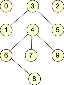 |
G2: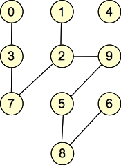 |
Wikipedia has a glossary of graph terms. The terms you should know are the following: vertices, edges, adjacency, incidence, directed/undirected, path, cycle, loop, multiedge, connected component, bipartite.
Wikipedia also has some pages that are less dense mathematically, which you may also find useful. Here is the page on graph theory.
Let's give some examples. Here are two graphs, which we will call G1 and G2:
| G1: |
G2: |
They are undirected graphs. G1 has four connected components and no cycles, while G2 has two connected components and one cycle. Both graphs are bipartite: with G1, the two sets of nodes are { 0, 1, 2, 5, 6, 7, 9 }, { 3, 4, 8 }. Other partitionings are possible (for example, nodes 0 and 2 can go into either set). For G2, the two sets are { 0, 1, 4, 7, 8, 9 }, { 2, 3, 5, 6 }. (You can put 4 into either set, but beyond that, the two sets are fixed).
Were we to add the edge (0, 1) to G2, it would no longer be bipartite.
If our adjacency lists contain indices of nodes, then the following table shows the adjacency list representation of the graph:
| Node | Adjacency list in G1 | Adjacency list in G2 |
| 0 | {} | { 3 } |
| 1 | { 3 } | { 2 } |
| 2 | {} | { 1, 9, 7 } |
| 3 | { 1, 5 } | { 0, 7 } |
| 4 | { 6, 7, 9 } | {} |
| 5 | { 3 } | { 9, 7 } |
| 6 | { 4, 8 } | { 8 } |
| 7 | { 4 } | { 2, 5 } |
| 8 | { 6 } | { 5, 6 } |
| 9 | { 4 } | { 2, 5 } |
With undirected graphs, we typically store each edge twice, which effectively makes the graph a directed graph. That is what we have done above.
You could, instead, have each node be its own data structure, and have each adjacency list be a vector of pointers to nodes. For example:
class Node {
  public:
    int num;
    vector <Node *> adj;
};
|
Then, G1 above would look as follows when it is stored in computer memory:
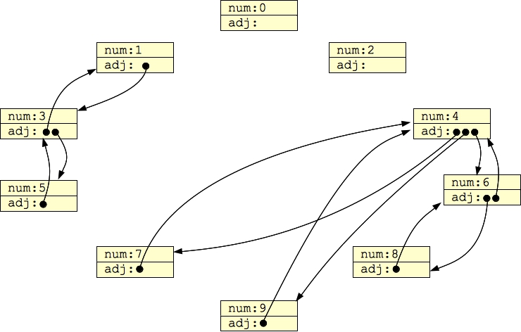 |
Here are the adjacency matrices for the two example graphs:
Adjacency Matrix for G1
     0  1  2  3  4  5  6  7  8  9
    -- -- -- -- -- -- -- -- -- --
 0 | 0  0  0  0  0  0  0  0  0  0
 1 | 0  0  0  1  0  0  0  0  0  0
 2 | 0  0  0  0  0  0  0  0  0  0
 3 | 0  1  0  0  0  1  0  0  0  0
 4 | 0  0  0  0  0  0  1  1  0  1
 5 | 0  0  0  1  0  0  0  0  0  0
 6 | 0  0  0  0  1  0  0  0  1  0
 7 | 0  0  0  0  1  0  0  0  0  0
 8 | 0  0  0  0  0  0  1  0  0  0
 9 | 0  0  0  0  1  0  0  0  0  0
|
Adjacency Matrix for G2
     0  1  2  3  4  5  6  7  8  9
    -- -- -- -- -- -- -- -- -- --
 0 | 0  0  0  1  0  0  0  0  0  0
 1 | 0  0  1  0  0  0  0  0  0  0
 2 | 0  1  0  0  0  0  0  1  0  1
 3 | 0  0  0  1  0  0  0  1  0  0
 4 | 0  0  0  0  0  0  0  0  0  0
 5 | 0  0  0  0  0  0  0  1  1  1
 6 | 0  0  0  0  0  0  0  0  1  0
 7 | 0  0  1  1  0  1  0  0  0  0
 8 | 0  0  0  0  0  1  1  0  0  0
 9 | 0  0  1  0  0  1  0  0  0  0
|
Because this is an undirected graph, each edge has two entries in the adjacency matrix. It also means that the adjacency matrices are symmetric around the diagonal of the matrix.
If we let |V| be the number of nodes, and |E| be the number of edges (we'll see why we use those terms later), then adjacency lists consume O(|E|) of memory, while adjacency matrices consume O(|V|2) of memory. For that reason, we typically use adjacency matrices either when the graphs are so small that the size of the matrix doesn't matter, or when the graph is very dense, which means that |E| is O(|V|2), and the matrix and list representations use roughly the same amount of memory.
V is a set of vertices, and E is a set of edges. (Yes, Wikipedia will tell you that technically, E is not a set, but that's one of those examples of Wikipedia pages being written by bored theoreticians. For now, call E a set.)
Because they are sets, you denote the size of V, and therefore the number of vertices as |V|. Similarly, the number of edges is |E|.
The specification of V and E defines the graph. For example, here is a mathematical definition of G1:
The mathematical representation can be very powerful, albeit a little terse and sometimes hard to read. For example, recall the binary heap implementation of priority queues (In the Priority Queue lecture notes). That data may be viewed as a graph, as it's clear where the nodes and edges are. Here's an example from that lecture:
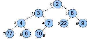 |
This lends itself to a beautiful mathematical definition:
When we implemented a maze in the disjoint set lecture, we were also implementing a graph. However, that graph was represented by a list of walls, which is neither an adjacency list or matrix. Instead, you can think of it as follows:
txt/g1.txt
NNODES 10 EDGE 4 9 EDGE 4 6 EDGE 4 7 EDGE 6 8 EDGE 3 5 EDGE 1 3 |
txt/g2.txt
NNODES 10 EDGE 5 9 EDGE 1 2 EDGE 5 8 EDGE 3 7 EDGE 2 7 EDGE 0 3 EDGE 5 7 EDGE 6 8 EDGE 2 9 |
I can specify the edges in any order.
When we did tree traversals in CS202, they are DFS's. With a preorder traversal, you do the activity before calling DFS recursively, and with a postorder traversal, you do the activity after calling DFS recursively. The inorder traversal is a DFS too, where you do the activity in the middle of the DFS calls.
This results in the following algorithm for determining connected components. First, you read in a graph. Then you set all visited fields to zero. Then you traverse all the nodes in the graph, and whenever you encounter one whose visited field is zero, you perform the connected component depth first search on it. The total number of depth first searches is equal to the number of connected components in the graph.
The code is in src/concomp.cpp. (I have a second implementation which has pointers in the adjacency lists rather than integers, because sometimes I write that in class instead. Please take a look at these notes to see that program, and an explanation of how it differs.)
In this program, we have separate classes for graphs and nodes. Graphs contain a vector of nodes (pointers to nodes, really). Each node has an adjacency list called edges, and this is a list of node numbers, as described above. The DFS is called Component_Count(), and it takes two parameters -- the node on which to perform the DFS (n), and the component number. The DFS uses a field component in each node as its visited field; however, instead of setting it to false initially, it is set to -1. And instead of setting it to true during the DFS, it is set to the component number.
The code is below. It is pretty straightforward:
#include <iostream>
#include <string>
#include <vector>
#include <stdlib.h>
using namespace std;

/* Each node is stored in one of these data structures.
   We are using adjacency lists to store edges, but instead
   of using the list data structure, we are using a vector.
   This is because it is space efficient and convenient. */

class Node {
  public:
    int id;                 // The node's number.
    vector <int> edges;     // Adjacency list, holding the
                            // numbers of the nodes to which
                            // this node is connected.
    int component;          // Component number.
};

/* This is the data structure for the graph. */

class Graph {
  public:
    vector <Node *> nodes;                    // All of the nodes.  nodes[i]->number is i
                                              // Note that it is a vector of pointers.
    void Component_Count(int index, int cn);  // This does the DFS to set components.
    void Print() const;                       // Print the graph.
};

// This is the DFS, where the component variable is used as the visited field.

void Graph::Component_Count(int index, int cn)
{
  Node *n;
  size_t i;

  n = nodes[index];
  if (n->component != -1) return;
  n->component = cn;
  for (i = 0; i < n->edges.size(); i++) Component_Count(n->edges[i], cn);
}

// The Print() function prints each node, its component number and its adjacency list.

void Graph::Print() const
{
  size_t i, j;
  Node *n;

  for (i = 0; i < nodes.size(); i++) {
    n = nodes[i];
    cout << "Node " << i << ": " << n->component << ":";
    for (j = 0; j < n->edges.size(); j++) {
      cout << " " << n->edges[j];
    }
    cout << endl;
  }
}

// The main() function reads in a graph, does the connected component
// determination, and then prints the graph.

int main()
{
  Graph g;
  string s;
  size_t nn, n1, n2, c;
  size_t i;
  Node *n;

  /* Read the number of nodes and create all of the nodes. */

  cin >> s;
  if (s != "NNODES") { cerr << "Bad graph\n"; exit(1); }
  cin >> nn;

  for (i = 0; i < nn; i++) {
    n = new Node;
    n->component = -1;
    n->id = i;
    g.nodes.push_back(n);
  }

  /* Read the edges. */

  while (!cin.fail()) {
    cin >> s >> n1 >> n2;
    if (!cin.fail()) {
      if (s != "EDGE") { cerr << "Bad graph\n"; exit(1); }
      g.nodes[n1]->edges.push_back(n2);
      g.nodes[n2]->edges.push_back(n1);
    }
  }

  /* Do the connected component analyses, and print the graph */

  c = 0;
  for (i = 0; i < g.nodes.size(); i++) {
    if (g.nodes[i]->component == -1) {
      c++;
      g.Component_Count(i, c);
     }
  }
  g.Print();

  return 0;
}
|
As we can see, it works fine on our two example files. Pay attention to the output. Each line prints a node, its connected component number, and its adjacency list. Make sure you understand the output and how it relates to the pictures.
UNIX> bin/concomp < txt/g1.txt
Node 0: 1:
Node 1: 2: 3
Node 2: 3:
Node 3: 2: 5 1
Node 4: 4: 9 6 7
Node 5: 2: 3
Node 6: 4: 4 8
Node 7: 4: 4
Node 8: 4: 6
Node 9: 4: 4
UNIX> bin/concomp < txt/g2.txt
Node 0: 1: 3
Node 1: 1: 2
Node 2: 1: 1 7 9
Node 3: 1: 7 0
Node 4: 2:
Node 5: 1: 9 8 7
Node 6: 1: 8
Node 7: 1: 3 2 5
Node 8: 1: 5 6
Node 9: 1: 5 2
UNIX>
The first call identifies the connected components as:
What's the running time? O(|V| + |E|). This covers two cases:
Cycle detection is another depth first search. Here we also set a visited field; however, if we now encounter a node whose visited field is set, we know that the node is part of a cycle, and we return that fact. Again, it's a simple search, and I put the relevant code below (src/cycledet0.cpp):
/* The structure of the graph is the same as the
   connected component problem. */

class Node {
  public:
    int id;
    vector <int> edges;
    int visited;
};

class Graph {
  public:
    vector <Node *> nodes;
    bool is_cycle(int index);    // Returns whether there is a cycle.
    void Print() const;
};

bool Graph::is_cycle(int index)
{
  Node *n;
  size_t i;

  n = nodes[index];
  if (n->visited) return true;
  n->visited = 1;
  for (i = 0; i < n->edges.size(); i++) {
    if (is_cycle(n->edges[i])) return true;
  }
  return false;
}

int main()
{
  ....

  for (i = 0; i < g.nodes.size(); i++) {
    if (!g.nodes[i]->visited) {
      if (g.is_cycle(i)) {
        cout << "There is a cycle reachable from node " << i << endl;
      } else {
        cout << "No cycle reachable from node " << i << endl;
      }
    }
  }
  return 0;
}
|
Note that unlike connected components, this procedure has a return value, and it uses that return value to truncate the search when a cycle is found.
When we run it, we see that it doesn't work correctly, as it says that g1 has a bunch of cycles, when we know that it doesn't:
UNIX> bin/cycledet0 < txt/g1.txt
No cycle reachable from node 0
There is a cycle reachable from node 1
No cycle reachable from node 2
There is a cycle reachable from node 4
There is a cycle reachable from node 6
There is a cycle reachable from node 7
There is a cycle reachable from node 8
UNIX>
Hmmm -- in src/cycledet1.cpp I put a print statement at the beginning of is_cycle():
UNIX> bin/cycledet1 < txt/g1.txt
Called is_cycle(0)
No cycle reachable from node 0
Called is_cycle(1)
Called is_cycle(3)
Called is_cycle(5)
Called is_cycle(3)
There is a cycle reachable from node 1
...
There's the bug. The program first visits node 0 and finds no cycle. Then it visits node 1 and recursively visits nodes 3 and 5. Since node 5 has an edge back to node 3, it detects a cycle there. How do we fix this bug?
One simple way is to include who calls is_cycle() as a parameter so that is_cycle() will not detect cycles that include the same edge twice. Here's the changed procedure and call from main() in src/cycledet2.cpp
bool Graph::is_cycle(int index, int from)
{
  Node *n;
  size_t i;

  n = nodes[index];
  if (n->visited) return 1;
  n->visited = 1;
  for (i = 0; i < n->edges.size(); i++) {
    if (n->edges[i] != from) {
      if (is_cycle(n->edges[i], index)) return 1;
    }
  }
  return 0;
}

main(int argc, char **argv)
{
  ...
  for (i = 0; i < g.nodes.size(); i++) {
    if (!g.nodes[i]->visited) {
      if (g.is_cycle(i, -1)) {
        cout << "There is a cycle reachable from node " << i << endl;
      } else {
        cout << "No cycle reachable from node " << i << endl;
      }

    }
  }
}
|
All works well now:
UNIX> bin/cycledet2 < txt/g1.txt
No cycle reachable from node 0
No cycle reachable from node 1
No cycle reachable from node 2
No cycle reachable from node 4
UNIX> bin/cycledet2 < txt/g2.txt
There is a cycle reachable from node 0
No cycle reachable from node 4
UNIX>
If you want to print the cycle, then you can start from when you first detect the cycle, and then stop when you reach the node from whence you detected the cycle. That's in src/cycledet3.cpp. Note, when I detect the cycle, I set the visited field to two. That is how I know when to stop printing and exit the program:
bool Graph::is_cycle(int index, int from)
{
  Node *n;
  size_t i;

  n = nodes[index];
  if (n->visited) {                // When we detect the cycle, set the node's
    n->visited = 2;                // visited field to two and return.
    cout << "Cycle: " << index;
    return true;
  }
  n->visited = 1;
  for (i = 0; i < n->edges.size(); i++) {
    if (n->edges[i] != from) {
      if (is_cycle(n->edges[i], index)) {   // If we have detected a cycle, then
        cout << " " << index;               // print the nodes in the cycle.
        if (n->visited == 2) {
          cout << endl;
          exit(1);
        }
        return true;
      }
    }
  }
  return false;
}
|
UNIX> cycledet3 < txt/g2.txt
Cycle: 7 5 9 2 7
UNIX>
For some of our examples, we are going to generate random undirected graphs. This is a relatively simple matter, but does take a little care. First, think about a file format format for our graphs. A simple format is to first specify the number of nodes and assume that the nodes are labeled with numbers from zero to the number of nodes minus one. Then we specify the edges by specifying the two nodes that each edge connects. That specification makes it easy to write code to read the graph, since you can allocate all the nodes after reading the first line.
There are other ways, of course, to represent graphs, which you will see in subsequent lectures and labs.
Our graph generation program bin/gen_graph takes two arguments: number of nodes and number of edges, and then it emits the number of nodes and generates the appropriate number of random edges. There are two pitfalls in writing bin/gen_graph. First is that you don't want to generate edges from a node to itself, and second is that you don't want to generate duplicate edges. The first pitfall is taken care of easily by checking to make sure that the second random node generated does not equal the first.
To address the second pitfall, we use a set. When we generate a random edge, we turn it into a string composed of the id of the smaller node followed by a space and then the id of the larger node. We check the set for that string, and if it is there, then we have a duplicate edge and must throw it out and try again.
The code is in src/gen_graph.cpp. Note it error checks to make sure that e is ≤ n(n-1)/2. Think about why:
#include <cstdio>
#include <iostream>
#include <string>
#include <set>
#include <cstdlib>
using namespace std;

int main(int argc, char **argv)
{
  int n;
  int e;
  int i;
  int n1, n2;
  set <string> edges;
  set <string>::iterator eit;
  string s;
  char edge[100];

  if (argc != 3) {
    cerr << "usage: ggraph n e\n";
    exit(1);
  }

  n = atoi(argv[1]);
  e = atoi(argv[2]);
|
  if (e > (n-1) * n / 2) {
    cerr << "e is too big\n";
    exit(1);
  }

  srand48(time(0));
  cout << "NNODES " << n << endl;
  for (i = 0; i < e; i++) {
    do {
      n1 = lrand48()%n;
      do n2 = lrand48()%n; while (n2 == n1);
      if (n1 < n2) {
        sprintf(edge, "%d %d", n1, n2);
      } else {
        sprintf(edge, "%d %d", n2, n1);
      }
      s = edge;
    } while (edges.find(s) != edges.end());

    edges.insert(s);

    cout << "EDGE " << s << endl;
  }
}
|
It works as it should. Here we generate two random graphs each with ten nodes.
UNIX> bin/gen_graph 10 6 > txt/g1.txt
UNIX> sleep 1
UNIX> bin/gen_graph 10 9 > txt/g2.txt
Here are the graph pictures and files:
|
txt/g1.txt
NNODES 10 EDGE 4 9 EDGE 4 6 EDGE 4 7 EDGE 6 8 EDGE 3 5 EDGE 1 3 |
txt/g2.txt
NNODES 10 EDGE 5 9 EDGE 1 2 EDGE 5 8 EDGE 3 7 EDGE 2 7 EDGE 0 3 EDGE 5 7 EDGE 6 8 EDGE 2 9 |
You'll note, g1 has six edges, four connected components and no cycles. G2 has nine edges, two connected components and one cycle (2,7,5,9,2).
(As an aside, is the above program really a good one? Ask youself, when is it good, and when is it bad? If you aren't sure of yourself, ask me in class.)