CS302 Lecture Notes - Network Flow Supplemental Lecture
Some extra help with Network Flow
- April 2, 2008. Latest revision, November, 2014.
- James S. Plank
- Directory: /home/plank/cs302/Notes/Netflow-All
This is an old lecture that I include now as supplemental material.
In this lecture, I give an example of calculating network flow with three different
path-finding algorithms. At the end, I show how to find the minimum cut.
Greedy Depth-First Search
The pathelogical example from lecture 1
highlights a problem -- choosing paths with little flow. One way to
combat this problem is to perform your DFS so that you prefer edges with a lot of flow to
edges with a little flow. You can implement that by having your adjacency lists be sorted by
flow, and then running a standard DFS on them. I'll show the augmenting paths that arise
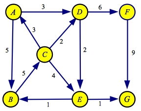
with this method on the example graph below. The source is A an the sink is G:
When we perform a greedy DFS on this graph, we start with edge from A to B
since its flow is greater than the edge from A to D. There is only one
edge leaving B. When we read node C, we traverse the edge to E, since
it has the maximum flow of C's three edges. Finally, E goes to G.
Thus, the first path we get is A->B->C->D->G
with a flow of one.
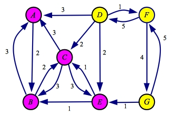
Below, I show the flow and residual graphs when this path is
processed. In the residual, the edges whose flow is reduced are colored red, and
the reverse edges are colored green:
| Flow 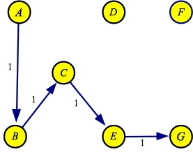
| Residual 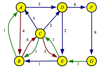
|
The next greedy path through the residual is A->B->C->D->F->G, with a flow of two:
| Flow 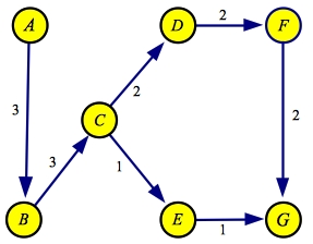
| Residual 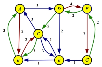
|
The last path is A->D->F->G with a flow of three. Here are the final flow and
residual graphs:
| Flow 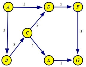
| Residual 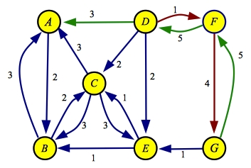
|
Finding the Maximum Flow Path through the Graph
Instead of using a depth-first search, you can use a modification of Dijkstra's
algorithm to find the path through the residual that has the maximum flow.
When processing a node, Dijkstra's algorithm traverses the node's edges, and
if shorter paths to any other nodes is discovered, the nodes are updated. At each
step, the node with the shortest known path is processed next.
The modification works as follows. When processing a node, again the algorithm
traverses the node's edges, and if paths with more flow to any other nodes are
discovered, then the nodes are updated. At each step, the node with the maximum
flow is processed next.
We'll work an example with the same graph as above:
The maximum flow path here is A->D->F->G with a flow of three:
| Flow 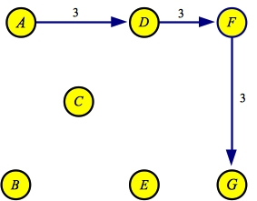
| Residual 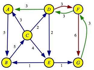
|
The next maximum flow path is A->B->C->D->F->G with a flow of 2:
| Flow 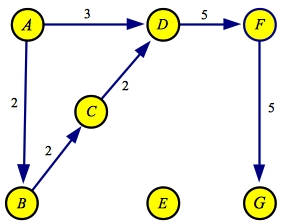
| Residual 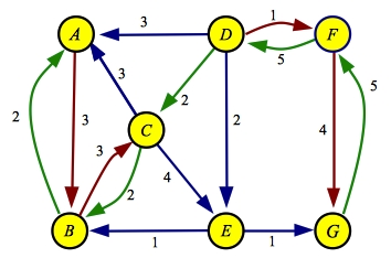
|
The final path is A->B->C->E->G with a flow of one:
| Flow
| Residual 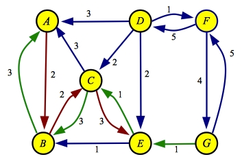
|
Edmonds-Karp: Finding the minimum hop path
Finally, the Edmonds-Karp algorithm uses a straightforward breadth-first search
to find the minimum hop path through the residual graph. This is equivalent to
treating the residual as an unweighted and performing a shortest path search on
it.
Again, we use the same graph as an example:
There are two minimum hop paths: A->D->E->G and A->D->F->F. Suppose
we process the former of these, with a flow of one:
| Flow 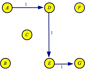
| Residual 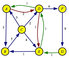
|
Now, there is only one minimum hop path through the residual: A->D->F->G, with a flow
of two:
| Flow 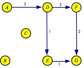
| Residual 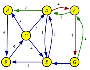
|
At this point, there are only two paths through the residual: A->B->C->D->F->G and
A->B->C->E->D->F->G. The first of these has fewer hops, so we process it.
It has a flow of two:
| Flow 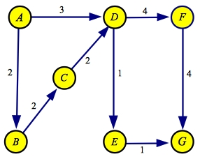
| Residual 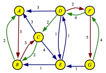
|
The final path through the residual is A->B->C->E->D->F->G with a flow of one. When
we process it, we get the same flow and residual graphs as the other two algorithms:
| Flow
| Residual 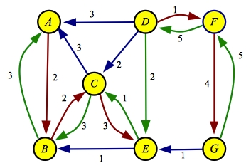
|
Bottom Lines
We've shown three ways to calculate the augmenting paths. Each way yields a different ordering
of augmenting paths; however, all three ways lead to the same flow and residual.
They differ in what they try to optimize.
- The greedy DFS and modified Dijkstra algorithms attempt to minimize the number of
paths that you find by finding paths with a lot of flow. They each have an expensive
component -- in greedy DFS, processing the residual graph is O(|V|log|V|) rather
than
O(|V|). In the modified Dijkstra, finding the augmenting path is
O(|E|log|V|) rather than O(|E|).
- Edmonds-Karp attempts to find a small number of paths, but its path-finding algorithm
is fast -- O(|E|) -- as is its residual processing algorithm, which is O(|V|).
There's no nice closed form solution for either the greedy DFS or the Modified Dijkstra
algorithm. When we evaluate performance, the greedy DFS is significantly slower, and
Modified Dijkstra runs on par with Edmonds-Karp. Edmonds Karp does have a closed
form running time: O(|V||E|2).
One thing that you should remember about network flow is that it is quite a bit slower than
all of the other graph algorithms we've studied so far.
Finding the Minimum Cut
As detailed in the
first network flow lecture, you can use
the final residual graph to find the minimum cut.
First, you find all nodes reachable from the source
in the residual graph. This is one set of nodes, which we color purple below:
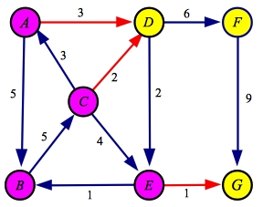
Now, in the original graph, we divide our nodes into two sets: the set determined above, and all of
the remaining nodes. They are drawn purple and yellow in the original graph below:
The minimum cut is composed of all the edges that go from the source set to the sink set. These are edges AD, CD and EG, which I've drawn in red above.
The sum of their capacities equals the maximum flow of six.