g1.txt:SOURCE S SINK T EDGE A B 5 EDGE A T 5 EDGE B T 8 EDGE C B 13 EDGE C D 10 EDGE D T 12 EDGE S A 10 EDGE S C 14 |
g1a.txt:SOURCE S SINK T EDGE D T 12 EDGE A T 5 EDGE S C 14 EDGE S A 10 EDGE C D 10 EDGE B T 8 EDGE A B 5 EDGE C B 13 |
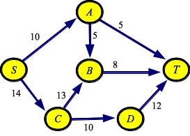 |
So, for example, below are two files that represent the graph from the First set of network flow lecture notes. They differ in the order in which they specify edges. Thus, the graph is the same, but the order of the adjacency lists will differ.
g1.txt:SOURCE S SINK T EDGE A B 5 EDGE A T 5 EDGE B T 8 EDGE C B 13 EDGE C D 10 EDGE D T 12 EDGE S A 10 EDGE S C 14 |
g1a.txt:SOURCE S SINK T EDGE D T 12 EDGE A T 5 EDGE S C 14 EDGE S A 10 EDGE C D 10 EDGE B T 8 EDGE A B 5 EDGE C B 13 |
|
I also have a program that generates random graphs, called src/makerandom.cpp. This program takes one or two arguments. The first argument is a number of nodes. The second number is an optional seed to srand48(). The program creates a random graph with one source, one sink, and the given number of other nodes. There is a random edge between every pair of nodes (in a random direction) with a random integer capacity between 1 and 10,000. There are edges from the source to random nodes with a 40% probability, and there are edges to the sink from random nodes with a 40% probability. Thus, this is a pretty dense graph which should be a challenge to our network flow programs.
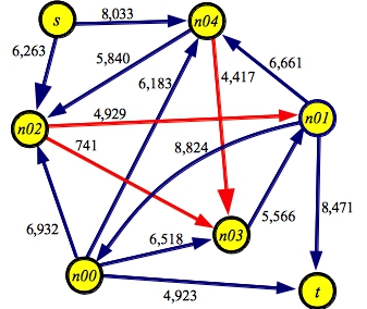
Below is an example of a graph made with makerandom 5. I think we can all agree that finding the maximum flow through this graph will be a bit of a challenge. To help you, I've colored the edges in the minimum cut red:
g5.txt:SOURCE s SINK t EDGE n00 t 4923 EDGE n01 n00 8824 EDGE n00 n02 6932 EDGE n00 n03 6518 EDGE n00 n04 6183 EDGE n01 t 8471 EDGE n02 n01 4929 EDGE n03 n01 5566 EDGE n01 n04 6661 EDGE s n02 6263 EDGE n02 n03 0741 EDGE n04 n02 5840 EDGE n04 n03 4417 EDGE s n04 8033 |
 |
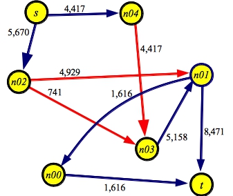
And here's a graph showing the maximum flow of 10,087
 |
These are written in an "old-school" manner, which will be useful for you to read-over so you can prepare for CS360. I may update them someday, but not this year...
My program has three basic classes: Node, Edge and Graph. Let's start with the Node and Edge classes:
class Node {
  public:
    string name;                    // The node's name
    vector <class Edge *> adj;      // The node's adjacency list in the residual graph.
    int visited;                    // A visited field for depth-first search.
};

class Edge {
  public:
    void Print() const;             // This prints the edge's name and residual flow.
    string name;                    // The edge's name (to store in the edge map).
    Node *n1;                       // The "from" node
    Node *n2;                       // The "to" node
    Edge *reverse;                  // The reverse edge, for processing the residual graph
    int original;                   // The original edge capacity.
    int residual;                   // The edge capacity in the residual graph.
};
|
Nodes are pretty simple. They have names, and adjacency lists. For now, we will represent the adjacency lists with vectors. Nodes also have a visited field, which helps us when we use DFS to find paths.
Edges are a little meatier. They have names, and pointers to the nodes that they connect. We store their original capacities and their residual capacities. If we wanted to maintain flow, we could do that too. However, I'm not doing that, simply to keep the program cleaner. When you do your lab, you're going to need to maintain the flow.
Each edge has a pointer to its reverse edge. This simplifies the task of processing the residual graph. I'm going to make sure that each edge always has a reverse edge, regardless of whether that reverse edge really exists in the residual graph. If the reverse edge really doesn't exist, I'm going to create it anyway, and give it an original and residual capacity of zero. When I "remove" an edge from the residual graph, I simply set its residual capacity to zero.
In this initial implementation, I'm going to have all edges go onto their nodes' adjacency lists, regardless of whether their capacities are zero. That makes the programming easier to begin with. We'll fix this later.
Finally, each edge has a name and a Print() method, which is useful, because there are several places where we print out edges.
You'll note, we're keeping pointers to nodes and edges. This is because there are several different places where we want to access nodes and edges, and to avoid making copies, we have exactly one copy of each node and edge, and we manipulate pointers to them.
Here is the definition of the Graph class:
class Graph {
  public:
     Graph();
     ~Graph();
     void Print() const;                 /* Print the graph to stdout. */
     string Verbose;                     /* G = print graph at each step.
                                            P = print augmenting paths at each step.
                                            B = Basic: print graph at beginning and end. */
     Node *Get_Node(const string &s);    /* Create a node, or return it if already created. */
     Edge *Get_Edge(Node *n1, Node *n2); /* Create an edge or return it if already created. */
     int MaxFlow();                      /* Do the max flow calculation for the graph. */
     int Find_Augmenting_Path();         /* Find and process an augmenting path. */

     bool DFS(Node *n);                  /* DFS to find an augmenting path - returns success. */
     vector <Edge *> Path;               /* The augmenting path. */

     int NPaths;                         /* Number of paths for the calculation. */
     int MaxCap;                         /* Maximum edge capacity */

     Node *Source;                       /* Source and sink node. */
     Node *Sink;

     vector <Node *> Nodes;              /* All of the nodes. */
     vector <Edge *> Edges;              /* All of the edges. */

     map <string, Node *> N_Map;         /* The nodes, keyed by name. */
     map <string, Edge *> E_Map;         /* The edges, keyed by name. */
};
|
There's quite a bit here. Let's get the simple things out of the way. There is a constructor, a destructor, and a Print() method. I keep a string Verbose, which lets me adjust what I print:
The next four fields are how I hold nodes and edges. I have a vector, which enables me to easily access every node and edge, and I have a map, which I only use when I'm reading in the file. The map lets me look up nodes and edges by name. (Note in 2023 -- When I shifted to C++-11, I should have changed this map to an unordered_map. So, if you were thinking "why isn't he using an unordered_map?" you are thinking correctly).
Get_Node() and Get_Edge() are really convenient procedures. They look up the node or edge in the relevant map, and if it's there, they return a pointer. If it's not there, then they create it, insert it into map, and return it.
The last three methods and Path are for doing the network flow calculation.
Node *Graph::Get_Node(const string &s)
{
  Node *n;

  if (N_Map.find(s) != N_Map.end()) return N_Map[s];

  n = new Node;
  n->name = s;
  n->visited = 0;
  N_Map[s] = n;
  Nodes.push_back(n);
  return n;
}
|
Edge *Graph::Get_Edge(Node *n1, Node *n2)
{
  string en;
  Edge *e;

  en = n1->name + "->";
  en += n2->name;

  if (E_Map.find(en) != E_Map.end()) return E_Map[en];
  e = new Edge;
  e->name = en;
  E_Map[en] = e;
  Edges.push_back(e);
  e->original = 0;
  e->residual = 0;
  e->n1 = n1;
  e->n2 = n2;
  e->reverse = NULL;
  return e;
}
|
The only real subtlety here is that I don't create reverse edges in Get_Edge(). Instead, I do it in the graph constructor.
The graph constructor is also straightforward. I'll include the code here, but I'm not going to explain it much:
Graph::Graph()
{
  string s, nn, nn2, en;
  int cap;
  Node *n1, *n2;
  Edge *e, *r;

  MaxCap = 0;
  Source = NULL;
  Sink = NULL;

  while (cin >> s) {
    if (s == "SOURCE" || s == "SINK") {   /* Set the source or sink (error checking for duplicates. */
      if (!(cin >> nn)) exit(0);
      n1 = Get_Node(nn);
      if (s == "SOURCE") {
        if (Source != NULL) { cerr << "Two sources.\n"; exit(1); }
        Source = n1;
      } else {
        if (Sink != NULL) { cerr << "Two sinks.\n"; exit(1); }
        Sink = n1;
      }
                                    /* When you read an edge, create it, potentially creating */
    } else if (s == "EDGE") {       /* the nodes, set the capacities and reverse edges. */
      if (!(cin >> nn >> nn2 >> cap)) exit(0);
      if (cap <= 0) exit(0);

      n1 = Get_Node(nn);
      n2 = Get_Node(nn2);
      e = Get_Edge(n1, n2);
      e->original += cap;
      e->residual += cap;
      if (e->residual > MaxCap) MaxCap = cap + 1;

      if (e->reverse == NULL) {  /* This means that the edge was just created */
        r = Get_Edge(n2, n1);
        e->reverse = r;
        r->reverse = e;
        n1->adj.push_back(e);
        n2->adj.push_back(r);
      }
    }
  }
  MaxCap *= 2;        /* This is because you can add flow in both directions (just trust me) */
  if (Source == NULL) { cerr << "No Source.\n"; exit(1); }
  if (Sink == NULL) { cerr << "No Sink.\n"; exit(1); }
}
|
When I call Get_Edge(), I check reverse to see if it's NULL. If it is, then I have just created the edge for the first time. That is when I create the reverse edge, and put both of them on their respective adjacency lists.
I also have a destructor, which deletes all of the nodes and edges. This is good form, because if I create an instance of a graph and then delete it, all of the memory associated with the graph will be released:
Graph::~Graph()
{
  int i;

  for (i = 0; i < Nodes.size(); i++) delete Nodes[i];
  for (i = 0; i < Edges.size(); i++) delete Edges[i];
}
|
You'll note that I don't have a copy constructor or assignment overload. I probably should, and have them throw errors, because the pointers mean that the defaults will not work.
The Print() method prints each node and its adjacency list, showing the name and residual flow on each edge. And the main() simply reads the graph and prints it if Verbose contains a 'B'. Here are both:
void Edge::Print()
{
  printf("[%s:%d]", name.c_str(), residual);
}

void Graph::Print()
{
  int i, j;
  Node *n;

  printf("Graph:\n");
  for (i = 0; i < Nodes.size(); i++) {
    n = Nodes[i];
    printf("  ");
    printf("Node: %s - ", n->name.c_str());
    for (j = 0; j < n->adj.size(); j++) n->adj[j]->Print();
    printf("\n");
  }
}
|
main(int argc, char **argv)
{
  Graph *G;
  int f;

  if (argc > 2) {
    cerr << "usage: netflow verbosity(BGP) - graph on stdin\n";
    exit(1);
  }

  G = new Graph();

  if (argc == 2) G->Verbose = argv[1];
  if (G->Verbose.find('B') != string::npos) G->Print();

  delete G;   /* Doing this just to make sure that the destructor works */
}
|
UNIX> netflow_skeleton B < g1.txt
Graph:
  Node: S - [S->A:10][S->C:14]
  Node: T - [T->A:0][T->B:0][T->D:0]
  Node: A - [A->B:5][A->T:5][A->S:0]
  Node: B - [B->A:0][B->T:8][B->C:0]
  Node: C - [C->B:13][C->D:10][C->S:0]
  Node: D - [D->C:0][D->T:12]
UNIX> netflow_skeleton B < g5.txt
Graph:
  Node: s - [s->n02:6263][s->n04:8033]
  Node: t - [t->n00:0][t->n01:0]
  Node: n00 - [n00->t:4923][n00->n01:0][n00->n02:6932][n00->n03:6518][n00->n04:6183]
  Node: n01 - [n01->n00:8824][n01->t:8471][n01->n02:0][n01->n03:0][n01->n04:6661]
  Node: n02 - [n02->n00:0][n02->n01:4929][n02->s:0][n02->n03:741][n02->n04:0]
  Node: n03 - [n03->n00:0][n03->n01:5566][n03->n02:0][n03->n04:0]
  Node: n04 - [n04->n00:0][n04->n01:0][n04->n02:5840][n04->n03:4417][n04->s:0]
UNIX>
Again, every edge has a reverse edge, and these edges are stored on the adjacency lists.
int Graph::MaxFlow()
{
  int mf, f;

  NPaths = 0;
  mf = 0;
  while (1) {
    f = Find_Augmenting_Path();
    mf += f;
    if (f == 0) return mf;
    NPaths++;
  }
}
|
The next method is Find_Augmenting_Path(). This calls DFS() to find an augmenting path from Source to Sink. DFS() returns 1 if it succeeds and 0 if it fails. If it succeeds, the path is in the vector Path. The order of the edges in Path should be immaterial here -- as long as all of the edges are in the vector, then Find_Augmenting_Path() can process it. As it turns out, DFS and all of the other implementations have the edges in reverse order. Fortunately, that's not important.
int Graph::Find_Augmenting_Path()
{
  int i, f;
  Edge *e;

  /* Clear visited fields, and the path. Then find an augmenting path with DFS. */

  for (i = 0; i < Nodes.size(); i++) Nodes[i]->visited = 0;
  Path.clear();
  if (Verbose.find('G') != string::npos) Print();
  if (DFS(Source)) {

    /* Calculate the flow through the path */

    f = MaxCap;
    for (i = 0; i < Path.size(); i++) {
      if (Path[i]->residual < f) f = Path[i]->residual;
    }

    /* The path is in reverse order, so we print the vector from back to front */

    if (Verbose.find('P') != string::npos) {
      printf("Path with flow %d: ", f);
      for (i = Path.size()-1; i >= 0; i--) Path[i]->Print();
      printf("\n");
    }

    /* Process the residual Graph */

    for (i = 0; i < Path.size(); i++) {
      e = Path[i];
      e->residual -= f;
      e->reverse->residual += f;
    }

    return f;
  }
  return 0;
}
|
After finding a path, Find_Augmenting_Path() does three things. First, it calculates the flow, then it optionally prints the path, and last, it processes the residual graph, removing flow from the forward direction and adding it to the reverse direction. This is all straightfoward, because we don't bother deleting edges with zero residual capacity from the adjacency lists.
All that's left is to find an augmenting path. Here is the depth-first search. It is a straightforward recursive DFS. The only important thing is that we need to ignore zero capacity edges, because we want to find paths with flow:
int Graph::DFS(Node *n)
{
  int i;
  Edge *e;

  if (n->visited) return 0;
  if (n == Sink) return 1;
  n->visited = 1;

  for (i = 0; i < n->adj.size(); i++) {
    e = n->adj[i];
    if (e->residual != 0) {
      if (DFS(e->n2)) {
        Path.push_back(e);
        return 1;
      }
    }
  }
  return 0;
}
|
We create the path whenever a recursive call returns 1. In other words, we create it when we have actually found a path to the sink.
Let's see how this works on our example graph, which I'll reproduce below:
g1.txt:SOURCE S SINK T EDGE A B 5 EDGE A T 5 EDGE B T 8 EDGE C B 13 EDGE C D 10 EDGE D T 12 EDGE S A 10 EDGE S C 14 |
g1a.txt:SOURCE S SINK T EDGE D T 12 EDGE A T 5 EDGE S C 14 EDGE S A 10 EDGE C D 10 EDGE B T 8 EDGE A B 5 EDGE C B 13 |
|
Because these two graph files create adjacency lists in different orders, they find different paths when calculating the maximum flow. The flow in both graphs is the same, however.
UNIX> netflow_dfs_v_no_delete PB < g1.txt
Graph:
  Node: S - [S->A:10][S->C:14]
  Node: T - [T->A:0][T->B:0][T->D:0]
  Node: A - [A->B:5][A->T:5][A->S:0]
  Node: B - [B->A:0][B->T:8][B->C:0]
  Node: C - [C->B:13][C->D:10][C->S:0]
  Node: D - [D->C:0][D->T:12]
Path with flow 5: [S->A:10][A->B:5][B->T:8]
Path with flow 5: [S->A:5][A->T:5]
Path with flow 3: [S->C:14][C->B:13][B->T:3]
Path with flow 10: [S->C:11][C->D:10][D->T:12]
Max flow is 23 - Paths: 4
Graph:
  Node: S - [S->A:0][S->C:1]
  Node: T - [T->A:5][T->B:8][T->D:10]
  Node: A - [A->B:0][A->T:0][A->S:10]
  Node: B - [B->A:5][B->T:0][B->C:3]
  Node: C - [C->B:10][C->D:0][C->S:13]
  Node: D - [D->C:10][D->T:2]
UNIX> netflow_dfs_v_no_delete PB < g1a.txt
Graph:
  Node: S - [S->C:14][S->A:10]
  Node: T - [T->D:0][T->A:0][T->B:0]
  Node: D - [D->T:12][D->C:0]
  Node: A - [A->T:5][A->S:0][A->B:5]
  Node: C - [C->S:0][C->D:10][C->B:13]
  Node: B - [B->T:8][B->A:0][B->C:0]
Path with flow 10: [S->C:14][C->D:10][D->T:12]
Path with flow 4: [S->C:4][C->B:13][B->T:8]
Path with flow 5: [S->A:10][A->T:5]
Path with flow 4: [S->A:5][A->B:5][B->T:4]
Max flow is 23 - Paths: 4
Graph:
  Node: S - [S->C:0][S->A:1]
  Node: T - [T->D:10][T->A:5][T->B:8]
  Node: D - [D->T:2][D->C:10]
  Node: A - [A->T:0][A->S:9][A->B:1]
  Node: C - [C->S:14][C->D:0][C->B:9]
  Node: B - [B->T:0][B->A:4][B->C:4]
UNIX>
It is not a bad idea for you to process these paths yourself to reinforce how to process the residual graph. To help you, you can run the program with "PG", and that lets you see the residual graph at each stage of the calculation.
To delete edges, I have each edge store an integer index, which is the index of the edge in the adjacency list. When you delete an edge, what you do is first swap it with the last edge in the node's adjacency list (adjusting that node's index). Then you call pop_back() to delete the edge from the adjacency list. I do this because it makes deletion constant time. What I don't want to do is, for example, move every edge over and then resize the vector, because that is not a constant time action.
There is an interesting implementational issue arising from (in my opinion) bad design of the STL. Because push_back() doesn't return an iterator to the new node (like it should), and because rbegin() returns a reverse_iterator, I use push_front() whenever I put a new edge onto an adjacency list. This is because I can now grab its iterator easily with begin().
UNIX> time netflow_dfs_v_no_delete < g200.txt
Max flow is 316197 - Paths: 35860
4.451u 0.013s 0:04.46 100.0%	0+0k 0+1io 0pf+0w
UNIX> time netflow_dfs_v_delete < g200.txt
Max flow is 316197 - Paths: 39037
1.485u 0.009s 0:01.49 99.3%	0+0k 0+0io 0pf+0w
UNIX> time netflow_dfs_list_pf < g200.txt
Max flow is 316197 - Paths: 205014
11.953u 0.022s 0:11.97 100.0%	0+0k 0+0io 0pf+0w
UNIX> time netflow_dfs_list_pb < g200.txt
Max flow is 316197 - Paths: 5389
0.361u 0.009s 0:00.37 97.2%	0+0k 0+0io 0pf+0w
UNIX> time netflow_dfs_edge_list < g200.txt
Max flow is 316197 - Paths: 39037
1.996u 0.011s 0:02.01 99.5%	0+0k 0+0io 0pf+0w
UNIX>
First, they all find the same flow of 316197. Yay.
Second, since I know no one looks at those numbers but me, here they are graphed:
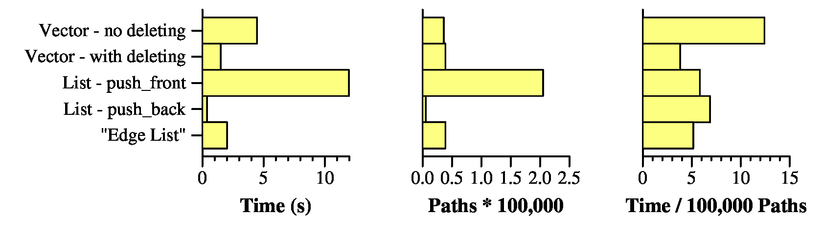 |
In terms of the two programs that use vectors, the one that deletes nodes is far preferable to the one that doesn't. That's because all of those zero capacity edges on the adjacency lists take up time in DFS(). The "Edge List" does a worse job than simply calling pop_back(), so we don't have to worry about that one any more. (also Yay).
What about the two list implementations -- that is amazing, isn't it? The one that calls push_front() took nearly 12 seconds, and the one that calls push_back() took the shortest amount of time of any of the implementations: Just 0.361 seconds.
The reason why has nothing to do with how the data structures are implemented. Instead, it has to do with the number of paths that are generated. The push_front() version generated 205,014 paths, while the push_back() version generated just 5,389. The other versions generated roughly 40,000 each. I want you to think about why the push_front() version generates lots of paths, and why the push_back() version generates few. It has to do with the fact that when you process a graph and you add an edge to an adjacency list, the edge is likely to have a small amount of capacity. So, if you put it in the front of a list, then you're more likely to find a new path with small flow rather than large. And small flow edges are bad (remember the pathelogical example from the first set of lecture notes).
Now, if you divide the running times by the number of paths (rightmost graph), then you get 0.000038 seconds per path with netflow_dfs_v_delete, and 0.000067 seconds per path with netflow_dfs_list_pb. So using a vector and deleting is the fastest way to process paths, when you normalize by the number of paths. We are therefore going to use src/netflow_dfs_v_delete.cpp as our starting point for the remaining implementations.