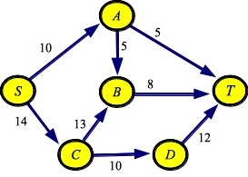
g1.txt:SOURCE S SINK T EDGE A B 5 EDGE A T 5 EDGE B T 8 EDGE C B 13 EDGE C D 10 EDGE D T 12 EDGE S A 10 EDGE S C 14 |
g1a.txt:SOURCE S SINK T EDGE D T 12 EDGE A T 5 EDGE S C 14 EDGE S A 10 EDGE C D 10 EDGE B T 8 EDGE A B 5 EDGE C B 13 |
 |
g1.txt:SOURCE S SINK T EDGE A B 5 EDGE A T 5 EDGE B T 8 EDGE C B 13 EDGE C D 10 EDGE D T 12 EDGE S A 10 EDGE S C 14 |
g1a.txt:SOURCE S SINK T EDGE D T 12 EDGE A T 5 EDGE S C 14 EDGE S A 10 EDGE C D 10 EDGE B T 8 EDGE A B 5 EDGE C B 13 |
|
g5.txt:SOURCE s SINK t EDGE n00 t 4923 EDGE n01 n00 8824 EDGE n00 n02 6932 EDGE n00 n03 6518 EDGE n00 n04 6183 EDGE n01 t 8471 EDGE n02 n01 4929 EDGE n03 n01 5566 EDGE n01 n04 6661 EDGE s n02 6263 EDGE n02 n03 0741 EDGE n04 n02 5840 EDGE n04 n03 4417 EDGE s n04 8033 |
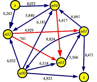 |
UNIX> netflow_dfs_greedy P < g1.txt
Path with flow 8: [S->C:14][C->B:13][B->T:8]
Path with flow 5: [S->A:10][A->T:5]
Path with flow 6: [S->C:6][C->D:10][D->T:12]
Path with flow 4: [S->A:5][A->B:5][B->C:8][C->D:4][D->T:6]
Max flow is 23 - Paths: 4
UNIX> netflow_dfs_greedy P < g5.txt
Path with flow 4923: [s->n04:8033][n04->n02:5840][n02->n01:4929][n01->n00:8824][n00->t:4923]
Path with flow 4417: [s->n02:6263][n02->n04:4923][n04->n03:4417][n03->n01:5566][n01->t:8471]
Path with flow 741: [s->n04:3110][n04->n02:5334][n02->n03:741][n03->n01:1149][n01->t:4054]
Path with flow 6: [s->n04:2369][n04->n02:4593][n02->n01:6][n01->t:3313]
Max flow is 10087 - Paths: 4
UNIX>
You should confirm the first paths in each of these graphs. Since edge SC has the largest capacity, that is the first one tried in the DFS. Then, since CB is C's largest edge, that is tried next, and since BT is B's only edge, that is the one that gets you to the sink. This is not the path with the largest flow (that is SCDT, but since the edge CB has bigger capacity than edge CD, it is processed first in the DFS.
Think about the cost tradeoffs of this algorithm versus a regular depth-first search. When you're processing the path, you are going to be doing insertions and deletions in the adjacency multimaps. Those are logarithmic time operations rather than constant time, so that will be slower than the regular DFS. We are hoping that the fewer number of paths will compensate.
Let's try the big 200-node graph:
UNIX> time netflow_dfs_greedy < g200.txt
Max flow is 316197 - Paths: 108
0.217u 0.009s 0:00.22 95.4%	0+0k 0+1io 0pf+0w
UNIX>
We have a winner! This beats all of our other DFS-based approaches.
You can do the same thing with flow. You maintain a set of nodes where you know the maximum flow to each of those nodes. Then you add the node that is not in the set, that has the highest flow to that set.
Let's put it another way -- with Dijkstra's shortest path algorithm, you maintain a multiset of nodes ordered by the shortest paths to the nodes. Instead, you are going to maintain a multiset of nodes ordered by the maximum flow to the nodes. It works in the same way.
The code is in netflow_dijkstra.cpp. This is the same as netflow_dfs_v_delete.cpp, but instead of DFS(), we have a method called Dijkstra(), which finds the maximum flow path. Below, I show the new Node variables to implement Dijsktra's algorithm and the Dijkstra() algorithm:
class Node {
  public:
    string name;
    vector <class Edge *> adj;
                                             /* These are added for Dijkstra's Algorithm: */
    int bestflow;                            /* The best flow discovered so far to this node. */
    class Edge *backedge;                    /* The edge from which this flow came. */
    multimap <int, Node *>::iterator qit;    /* If I'm on the queue, an iterator to my place. */
};


int Graph::Dijkstra()
{
  multimap <int, Node *> Q;     /* Here's the sorted list of best flow to nodes */
  Node *n;                      /* The node that I'm processing from the back of Q. */
  int f;                        /* When I'm processing n, this is the flow to n. */
  Edge *e;                      /* I process each edge from n */
  Node *t;                      /* This is the node that e goes to: e is (n,t) */
  int nf;                       /* This is the flow to t if I go through n.  If it's better than
                                   t's current best flow, I'll delete t from Q and put it back
                                   on Q with this flow. */

  multimap <int, Node *>::iterator qit;
  int i;

  for (i = 0; i < Nodes.size(); i++) Nodes[i]->bestflow = 0;

  /* Start by putting the Source onto the queue with infinite flow. */

  Source->backedge = NULL;
  Source->bestflow = MaxCap;
  Source->qit = Q.insert(make_pair(MaxCap, Source));

  /* Now process the Queue.
     Always process the last element (that's the one with the most flow). */

  while(!Q.empty()) {

    /* Grab the last element and delete it */
    f = Q.rbegin()->first;
    n = Q.rbegin()->second;
    Q.erase(n->qit);

    /* If we're at the sink, we're done.
       Create the path by traversing backedges back to the source. */

    if (n == Sink) {
      while (n != Source) {
        Path.push_back(n->backedge);
        n = n->backedge->n1;
      }
      return 1;
    }

    /* Otherwise, process each of n's edges, and if the path through n to t
       has better flow than t's current flow, then delete t from Q if it's
       there, and insert t into Q with this new flow. */

    for (i = 0; i < n->adj.size(); i++) {
      e = n->adj[i];
      t = e->n2;
      nf = (e->residual < f) ? e->residual : f;
      if (nf > t->bestflow) {
        if (t->bestflow != 0) Q.erase(t->qit);
        t->backedge = e;
        t->bestflow = nf;
        t->qit = Q.insert(make_pair(nf, t));
      }
    }
  }

  /* Return 0 if there's no path to the sink. */

  return 0;
}
|
As before, let's see it running on our two example graphs:
UNIX> netflow_dijkstra P < g1.txt
Path with flow 10: [S->C:14][C->D:10][D->T:12]
Path with flow 5: [S->A:10][A->T:5]
Path with flow 5: [S->A:5][A->B:5][B->T:8]
Path with flow 3: [S->C:4][C->B:13][B->T:3]
Max flow is 23 - Paths: 4
UNIX> netflow_dijkstra P < g5.txt
Path with flow 4929: [s->n02:6263][n02->n01:4929][n01->t:8471]
Path with flow 4417: [s->n04:8033][n04->n03:4417][n03->n01:5566][n01->n00:8824][n00->t:4923]
Path with flow 741: [s->n04:3616][n04->n02:5840][n02->n03:741][n03->n01:1149][n01->t:3542]
Max flow is 10087 - Paths: 3
UNIX>
As you see, with g1.txt, the output differs from the greedy DFS, because this one actually finds the maximum flow path at each step. Interestingly, with g5.txt, the two produce paths with the same flow, but the paths are different.
When we try it on the 200-node graph, we get the best time yet, with just 76 paths:
UNIX> time netflow_dijkstra < g200.txt
Max flow is 316197 - Paths: 76
0.154u 0.008s 0:00.47 31.9%	0+0k 0+1io 0pf+0w
UNIX>
As with the greedy DFS, let's think about the tradeoffs of this algorithm. With greedy DFS, we made processing the residual more expensive, because you had to insert and delete edges from the adjacency multimaps. Here, processing the residual is back to being cheap, involving constant time operations. The expense is in finding the paths, which is O(|E|log|V|) at each step, rather than O(|E|). To compensate for that expense, we are finding far fewer paths, since we find the maximum flow path at each step.
This is called the "Edmonds-Karp" algorithm, and its overall running time is (|V||E|2).
I don't show the program that implements it, because that's what you are going to implement in your lab. However, it is easier than the previous program, since it is a simply BFS. Here it is on our two example graphs:
UNIX> netflow_edmonds_karp P < g1.txt
Path with flow 5: [S->A:10][A->T:5]
Path with flow 5: [S->A:5][A->B:5][B->T:8]
Path with flow 3: [S->C:14][C->B:13][B->T:3]
Path with flow 10: [S->C:11][C->D:10][D->T:12]
Max flow is 23 - Paths: 4
UNIX> netflow_edmonds_karp P < g5.txt
Path with flow 4929: [s->n02:6263][n02->n01:4929][n01->t:8471]
Path with flow 741: [s->n02:1334][n02->n03:741][n03->n01:5566][n01->t:3542]
Path with flow 2801: [s->n04:8033][n04->n03:4417][n03->n01:4825][n01->t:2801]
Path with flow 1616: [s->n04:5232][n04->n03:1616][n03->n01:2024][n01->n00:8824][n00->t:4923]
Max flow is 10087 - Paths: 4
UNIX>
The algorithm is interesting because it works on the structure of the graph rather than its flow, but in doing so, improves the number of paths drastically from DFS. Here it is on the big, 200-node graph.
UNIX> time netflow_edmonds_karp < g200.txt
Max flow is 316197 - Paths: 176
0.134u 0.008s 0:00.14 92.8%	0+0k 0+0io 0pf+0w
UNIX>
Interesting, no? More paths, but faster path-finding make for a (slightly) faster algorithm.
 |
Ok, I lied above -- I stopped running some of the implementations (e.g. netflow_dfs_list_pf) above a certain graph size, because it's pretty obvious how they are scaling. The trends follow the explanation above. The three path-finding algorithms described in this lecture perform the best, and there's no real clear winner between the modified Dijkstra and Edmonds-Karp. It is interesting that the Edmonds-Karp curve is less jaggedy than the modified Dijkstra. Perhaps you can come up with a good explanation for that. It has to do with the structure of the graph.
Now take a look at the average number of augmenting paths processed by each algorithm:
 |
This is as we would expect. With the exception of the greedy DFS, the DFS algorithms generate way too many paths, as they don't put any effort into finding smart paths. The other three algorithms do a much better job at reducing the number of paths.
BTW, you can't see the curve for netflow_dfs_edge_list, because it is identical to netflow_dfs_v_delete.
Is it surprising to you that Edmonds-Karp runs so fast, yet is the worst of the three in terms of number of paths? It shouldn't be -- remember the running times of the various components:
| Finding the path | Processing the residual graph | |
| Greedy DFS | O(|E|) | O(|V|log(|V|)) |
| Modified Dijkstra | O(|E|log(|V|)) | O(|V|) |
| Edmonds-Karp | O(|E|) | O(|V|) |