 |
In include/pqueue.hpp, I define an interface for a priority queue which holds doubles. Then I define class definitions for two implementations:
#include <vector>
#include <set>

/* The Main Priority Queue Interface. */

class PQueue {
  public:
    virtual ~PQueue() {};
    virtual void    Push(double d) = 0;
    virtual double  Pop()          = 0;
    virtual size_t  Size() const   = 0;
    virtual bool    Empty() const  = 0;
    virtual void    Print() const  = 0;
};
|
/* PQueueSet: Implementing the priority
   queue with a multiset */

class PQueueSet : public PQueue {
  public:
    void    Push(double d);
    double  Pop();
    size_t  Size() const;
    bool    Empty() const;
    void    Print() const;

    PQueueSet();
  protected:
    std::multiset <double> elements;
};
|
/* PQueueHeap: Implementing the priority
   queue with a binary heap.  You'll note
   that there is a second constructor
   here that creates the priority queue
   from a vector of doubles. */

class PQueueHeap : public PQueue {
  public:
    void    Push(double d);
    double  Pop();
    size_t  Size() const;
    bool    Empty() const;
    void    Print() const;

    PQueueHeap();
    PQueueHeap(const std::vector <double> &init);
  protected:
    std::vector <double> h;
    void Percolate_Down(size_t index);
};
|
You'll note that there is an extra constructor in the heap implementation. This is a constructor that creates a priority queue from an unsorted vector of doubles. We'll discuss that more below.
#include <cstdio>
#include <iostream>
#include <cstdlib>
#include "pqueue.hpp"
using namespace std;

/* Using a multiset to implement the priority queue makes
   most of these methods really simple.  The first four
   here are one-liners: */

        PQueueSet::PQueueSet()    { }
void    PQueueSet::Push(double d) { elements.insert(d); }
size_t  PQueueSet::Size() const   { return elements.size(); }
bool    PQueueSet::Empty() const  { return elements.empty(); }

/* Print() is straightfoward. */

void PQueueSet::Print() const
{
  multiset <double>::const_iterator hit;

  for (hit = elements.begin(); hit != elements.end(); hit++) {
    if (hit != elements.begin()) cout << " ";
    cout << *hit;
  }
  cout << endl;
}
|
/* With Pop(), we error check, and then if the multiset
   is not empty, we return the first element, and erase
   it from the multiset. */

double PQueueSet::Pop()
{
  multiset <double>::iterator hit;
  double retval;

  if (elements.empty()) {
    throw (string) "Called Pop() on an empty PQueue";
  }
  hit = elements.begin();
  retval = *hit;
  elements.erase(hit);
  return retval;
}
|
To test, I have written two simple programs that use Priority Queues. The first is src/add_5.cpp. It creates an insteance of the PQueue and then prompts the user for five numbers. It pushes them onto the priority queue and then prints the queue. It reads its command line argument to determine whether to use the multiset implementation ('s') or the heap implementation ('h').
#include "pqueue.hpp"
#include <iostream>
#include <cstdlib>
#include <cstdio>
using namespace std;

int main(int argc, char **argv)
{
  PQueue *pq;
  int i;
  double d;

  /* Construct the proper implementation of the priority queue. */

  if (argc != 2 || (argv[1][0] != 's' && argv[1][0] != 'h')) {
    fprintf(stderr, "usage: add_5 s|h\n");
    exit(1);
  }

  switch (argv[1][0]) {
    case 's': pq = new PQueueSet(); break;
    case 'h': pq = new PQueueHeap(); break;
    default:  exit(1);
  }
|
  /* Prompt for five numbers.
     Push them and print the PQueue. */

  cout << "Enter five numbers.\n";

  for (i = 0; i < 5; i++) {
    if (!(cin >> d)) exit(1);
    pq->Push(d);
  }
  pq->Print();
  return 0;
}
|
When we run bin/add_5 on the multiset implementation, the numbers are sorted, because the multiset sorts them:
UNIX> bin/add_5 s
Enter five numbers.
3 5 2 4 1
1 2 3 4 5
UNIX>
The second program is src/pq_sort.cpp. This program reads doubles from standard input and sorts them using a priority queue. Like bin/add_5 it uses its command line argument to determine which implementation to use:
#include "pqueue.hpp"
#include <iostream>
#include <cstdlib>
#include <cstdio>
using namespace std;

int main(int argc, char **argv)
{
  PQueue *pq;
  double d;
  string imps;
  vector <double> v;

  /* Error check, and then create the pq with either the set or heap implementation. */

  imps = "shl";
  if (argc != 2 || imps.find(argv[1][0]) == string::npos) {
    fprintf(stderr, "usage: pqueue_sort c where c is a character in %s\n", imps.c_str());
    exit(1);
  }

  switch (argv[1][0]) {
    case 's': pq = new PQueueSet(); break;
    case 'h': pq = new PQueueHeap(); break;
    case 'l': pq = NULL; break;
    default:  exit(1);
  }

  /* With 's' and 'h', simply read and push onto the heap.  With 'l', read everything
     into a vector and then construct the heap from the vector. */

  if (pq == NULL) {
    while (cin >> d) v.push_back(d);
    pq = new PQueueHeap(v);
  } else {
    while (cin >> d) pq->Push(d);
  }

  /* Popping everything sorts the doubles. */

  while (!pq->Empty()) cout << pq->Pop() << endl;

  return 0;
}
|
Let's test it on the multiset:
UNIX> head -n 5 txt/input.txt
782.678
270.576
447.465
501.138
714.567
UNIX> head -n 5 txt/input.txt | bin/pq_sort s
270.576
447.465
501.138
714.567
782.678
UNIX> wc txt/input.txt
    1000    1000    7885 txt/input.txt
UNIX> bin/pq_sort s < txt/input.txt > txt/output1.txt
UNIX> sort -n input.txt > txt/output2.txt
UNIX> diff txt/output1.txt txt/output2.txt
UNIX>
Now, time to learn about binary heaps:
|
The other property of a heap is that the value of each node must be less than or equal to all of the values in its subtrees. That's it. Below are two examples of heaps:
 |
 |
That second one has duplicate values (two sixes), but that's ok. It still fits the definition of a heap.
Below are three examples of non-heaps:
 The 10 node is not smaller than the values in its subtrees. |
 Not a complete tree. |
 The last row is not filled from left to right. |
When we push a value onto a heap, we know where the new node is going to go. So we insert the value there. Unfortunately, that may not result in a new heap, so we adjust the heap by "percolating up." To percolate up, we look at the value's parent. If the parent is smaller than the value, then we can quit -- we have a valid heap. Otherwise, we swap the value with its parent, and continue percolating up.
Below we give an example of inserting the value 2 into a heap:
| Start
|
Put 2 into the new node and percolate up.
|
| Continue percolating, since 2 is less than 3.
|
Now we stop, since 1 is less than 2.
|
To pop a value off a heap, again, we know the shape of the tree when we're done -- we will lose the rightmost node on the last level. So what we do is put the value in that node into the root (we will return the old value of the root as the return value of the Pop() call). Of course, we may not be left with a heap, so as in the previous example, we must modify the heap. We do that by "Percolating Down." This is a little more complex than percolating up. To percolate down, we check a value against its children. If it is the smallest of the three, then we're done. Otherwise, we swap it with the child that has the minimum value, and continue percolating down.
As before, an example helps. We will call Pop() on the last heap above. This will return 1 to the user, and will delete the node holding the 7, so we put the value 7 into the root and start percolating down:
| Start
|
Swap 7 and 2
|
| Swap 7 and 3. We're Done.
|
If we think about running time complexity, obviously the depth of a heap with n elements is log2(n). Thus, Push() and Pop() both run with O(log(n)) complexity. This is the exact same as using a multiset above. So why do we bother?
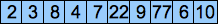
The answer is that even though the two have the same running time complexity, the heap implementation is more efficient. Since we always add and subtract elements to and from the end of the heap, we may implement the heap as a vector. The root is at index 0, the nodes at the next level are at indices 1 and 2, etc. For example, we show how the final heap above maps to a vector:
 |
 |
When we Push() an element onto the heap, we perform a push_back() on the vector, and then we percolate up. When we Pop() an element off the heap, we store the root, replace it with the last element, call pop_back() on the vector, and percolate down starting at the root. A quick inspection of the indices shows that:
/* With Push(), we append the new element to the
   end of the vector, and then percolate up. */

void PQueueHeap::Push(double d)
{
  int i, parent;
  double tmp;

  /* Put the element at the end of the vector. */

  h.push_back(d);

  /* And then percolate up.  i is always
     pointing to the newly added element. */

  i = h.size()-1;
  while (1) {
    if (i == 0) return;
    parent = (i-1)/2;
    if (h[parent] > h[i]) {
      tmp = h[i];
      h[i] = h[parent];
      h[parent] = tmp;
      i = parent;
    } else {
      return;
    }
  }
}
|
I have implemented Percolate_Down as a separate protected method, because it is used in two places. The first is Pop(), which moves the last element to the root of the tree and percolates down. Here is the code for both Percolate_Down(), Pop() and Print(). Percolate_Down() has to test a few cases, depending on whether there is a right child, or whether the right child's value is less than the left child's value.
/* I have implemented Percolate_Down as a separate
   protected method, because it is used in two
   places: Pop() and the vector constructor. */

void PQueueHeap::Percolate_Down(size_t index)
{
  size_t lc, rc;
  double tmp;

  /* lc is the left child, and
     rc is the right child. */

  while (1) {
    lc = index*2+1;
    rc = lc+1;

    /* If index is on the bottom of the heap,
       then return, because we can't
       percolate any more. */

    if (lc >= h.size()) return;

    /* With this code, either there is no
       right child, or the left child is
       smaller than the right child.  In
       this case, you need to compare the
       element at index with the left child. */

    if (rc == h.size() || h[lc] <= h[rc]) {
      if (h[lc] < h[index]) {
        tmp = h[lc];
        h[lc] = h[index];
        h[index] = tmp;
        index = lc;
      } else {
        return;
      }

    /* Otherwise, we compare the element at
       index with the right child. */

    } else if (h[rc] < h[index]) {
      tmp = h[rc];
      h[rc] = h[index];
      h[index] = tmp;
      index = rc;
    } else {
      return;
    }
  }
}
|
/* With Pop(), after we error check, we
   move the last element to the root of
   the heap, and percolate down. */

double PQueueHeap::Pop()
{
  double retval;

  if (h.empty()) {
    throw (string) "Called Pop() on an empty PQueue";
  }
  retval = h[0];
  h[0] = h[h.size()-1];
  h.pop_back();
  if (h.size() == 0) return retval;
  Percolate_Down(0);
  return retval;
}

/* The vector constructor calls Percolate_Down()
   on all non-leaf elements, going from the bottom
   of the heap to the top. */

PQueueHeap::PQueueHeap(const vector <double> &v)
{
  int i;

  h = v;

  for (i = (int) h.size()/2-1; i >= 0; i--) Percolate_Down(i);
}

/* Print is straightforward. */

void PQueueHeap::Print() const
{
  size_t i;

  for (i = 0; i < h.size(); i++) {
    if (i != 0) cout << " ";
    cout << h[i];
  }
  cout << endl;
}
|
Let's double-check ourselves with bin/add_5:
UNIX> bin/add_5 h
Enter five numbers.
3 5 2 4 1
1 2 3 5 4
UNIX> bin/add_5 h
Enter five numbers.
5 4 3 2 1
1 2 4 5 3
UNIX>
In the first call, we don't need to do any percolating when we insert elements into the heap. Thus, the vector has the values in order. In the second call, the five add calls each percolate the new value to the root of the heap:
 |
 |
 |
 |
 |
To verify that percolating down works, let's compare pq_sort with the multiset implementation:
UNIX> head -n 5 txt/input.txt | bin/pq_sort h
270.576
447.465
501.138
714.567
782.678
UNIX> bin/pq_sort h < txt/input.txt > txt/output3.txt
UNIX> diff txt/output1.txt txt/output3.txt
UNIX>
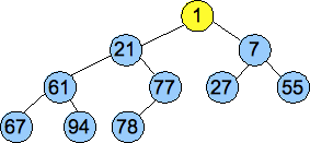
Below is an example. Here's the vector that we want to turn into a heap:
| 77 | 21 | 55 | 94 | 1 | 27 | 7 | 67 | 61 | 78 |
We convert the vector into a tree, as pictured below, and then we call Percolate_Down() on nodes of each successively higher level. These are the nodes pictured in yellow. By the time we get to the root, we have created a valid heap:
 |
 |
 |
 |
To analyze the running time complexity, we need a little math. Suppose our tree is complete at each level. The tree has n nodes, and thus its depth is log(n). The worst case performance of Percolate_Down() for a node at level i is log(n)-i. Thus, the performance of Percolate_Down() for a node at the bottom level is 1; for a node at the penultimate level, it is 2, etc.
The bottom level contains (n+1)/2 nodes, which is roughly n/2. Thus, all of the Percolate_Down()'s take (1)(n/2) = n/2 operations. At the next level, there are n/4 nodes, whose Percolate_Down()'s take 2 operations each. Thus, all of them take 2n/4. At the next level, there are n/8 nodes whose Percolate_Down()'s take 3 operations each. Thus, all of them take 3n/8. Do you see the pattern? To help you, try the animated gif in img/vector.gif, which shows the percolate down's for a heap with 511 elements.
The creation of the heap can be converted into a summation:
 |
To figure out what that second summation is, let's first write a quick C++ program to calculate its value for the first 15 values of n. The code is below (src/formula.cpp), and to the right, we show its output:
#include <iostream>
using namespace std;

int main()
{
  double num, den, total, n;

  num = 1;
  den = 2;
  total = 0;

  for (n = 0; n < 15; n++) {
    total += (num/den);
    num++;
    den *= 2;
    cout << total << endl;
  }
}
| UNIX> bin/formula 0.5 1 1.375 1.625 1.78125 1.875 1.92969 1.96094 1.97852 1.98828 1.99365 1.99658 1.99817 1.99902 1.99948 UNIX> |
Looks like it converges to 2. Let's analyze it mathematically. Consider the following sum:
 |
Now, let's consider the equation G - G/2:
 |
From high school math, we know that this last summation equals one, so G - G/2 = 1, which means that G = 2.
PQueueHeap::PQueueHeap(const vector <double> &v)
{
  int i;

  h = v;

  for (i = (int) h.size()/2-1; i >= 0; i--) Percolate_Down(i);
}
|
That was simple, wasn't it? We test performance below:
UNIX> bin/genrandom 1000 | bin/pq_sort s > /dev/null
UNIX>
If we try to time this with time, we see no output:
UNIX> time bin/genrandom 1000 | bin/pq_sort s > /dev/null
UNIX>
That's because time's output is also going to /dev/null. To fix this, we have time execute a subshell:
UNIX> time sh -c "bin/genrandom 1000 | bin/pq_sort s > /dev/null"
0.009u 0.005s 0:00.01 0.0%	0+0k 0+0io 0pf+0w
UNIX>
Great -- now we can write a shell script called scripts/bigtest_1.sh, which calls all three implementations with input sizes ranging from 1000 to 100,000:
UNIX> sh scripts/bigtest_1.sh | head
s 1000 0.00
s 2000 0.01
s 3000 0.02
s 4000 0.02
s 5000 0.02
s 6000 0.04
s 7000 0.04
s 8000 0.05
s 9000 0.05
s 10000 0.05
UNIX>
It prints out the implementation, the number of doubles and the wall clock time in seconds (MacBook Pro in 2018). The full data is in txt/test-data1.txt. I graph it below (using jgraph - scripts/sort_test1.jgr):
 |
That graph sucks. The main reason is the squiggly lines -- what they indicate is that the individual data points have some variance, and that we should run more than one run per test, averaging the results. Still, if we ignore the squiggly lines, we draw two conclusions:
I've written a testing program called src/massive_create.cpp, which takes three command line arguments:
I've also changed my shell script. For each test, it runs bin/massive_create with i iterations, where i * n = 10,000,000. That gives me running times on the order of .5 seconds per test. I ran this on the Linux box in my office (so that I'm not timing the 500 other things that my Macbook is doing right now), and varied the number of elements from 10,000 to 1,000,000 (just 100,000 for the multiset).
 |
Those jumps in the red lines are interesting, aren't they? I'll talk about them below.
That's a BIG difference, isn't it? Look at the values on the axes -- these tests are running roughly 100 times faster than the previous ones! Not only are the lines smoother, but you can very clearly see the performance improvements between multiset and heap, and from the two different constructors.
What should you take from this? First, that experimental computer science research can be very tricky. We had a simple goal: to demonstrate that a O(n) algorithm runs faster than a O(n(log(n))) one. We tried an obvious solution, and we couldn't use it because we weren't really testing what we wanted to test. When we rewrote our testing programs to do a better job of removing the noise from the experiment, we were able to demonstrate improved performance.
Second, the O(n) algorithm is indeed faster.
The first question you should ask yourself is whether those jumps are due to instruction count or memory. When I see curves like that, I think "memory." So, I instrumented pqueue_heap.cpp to keep track of the times it looks at an element of v in Push(). That is a rough estimate of instruction count. If you take a look at a graph of that, you'll see that the curve is smooth:
 |
That is a hint that it's not instruction count that is causing the jumps.
Take a look at the following graphs. In these, I have instrumented the programs so that they keep track of the elements of v that they access in each call to either Percolate_Down(), or Push(). Here's the graph for creating the heap by repeatedly calling Push(). Time goes from top to bottom.
 |
And here's the graph for creating the heap from the vector by repeatedly calling Percolate_Down():
 |
Can you see why the first graph would cause jumps with fixed-sized caches, and the second would not? This would be a great exercise for a cache modeling assignment. We can talk about it in class when we have the time. Or, if I take the time to write about it, I'll do so for you.


