 |
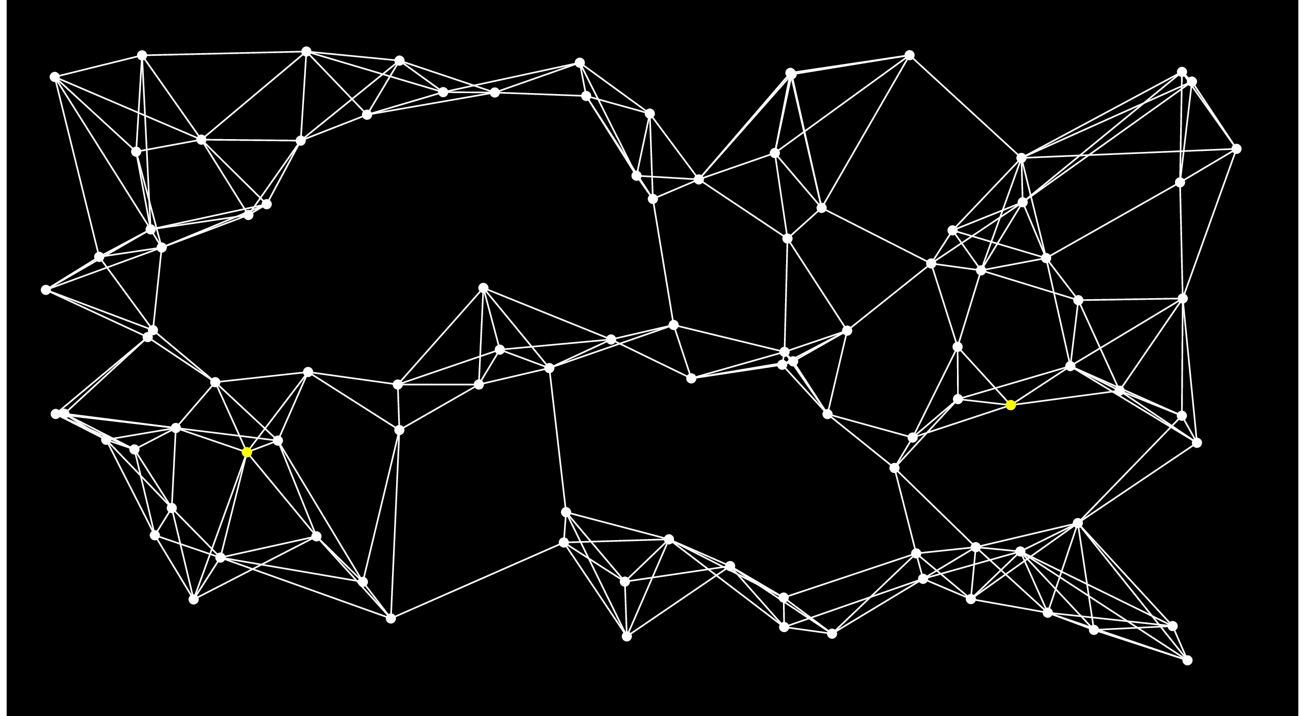
Let's pause here for an example. Let's consider the following graph, where the Start node is the yellow one on the left, and the End node is the one on the right:
|
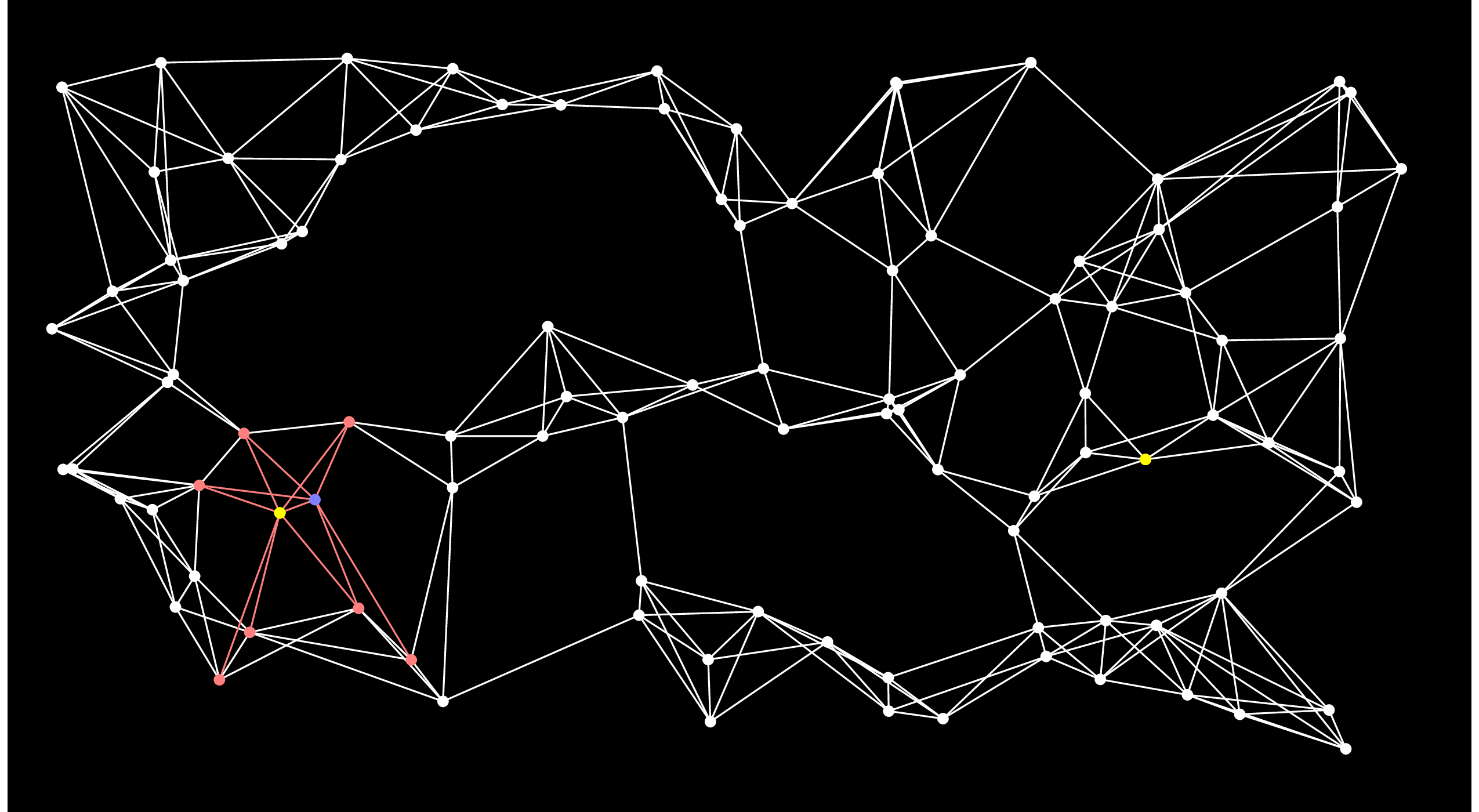
On the first step of Dijkstra's algorithm, we add all of the nodes directly connected to Start to the open set. I'll do that by coloring the edges and nodes red:
 |
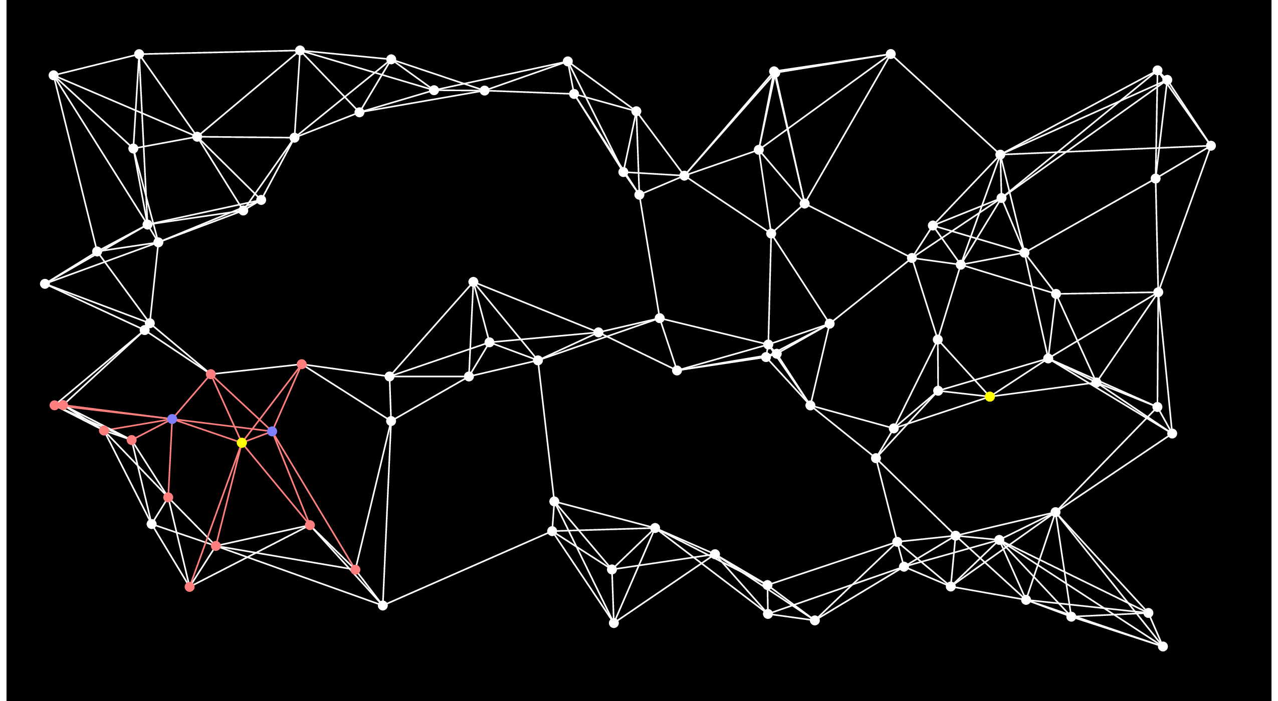
The nodes in the open set are ordered by their distance to Start. What Dijkstra's algorithm does is select the closest node in the ordered set -- we know that there is no node in the open set that is closer, so we can remove the node from the open set and add it to the closed set. I'll show that by coloring the node blue. We then traverse the node's adjacency list and if it is connected to any nodes that aren't in the open set, then it adds them to the open set. If it is connected to a node that is in the open set, then it considers that currently best known distsnce from Start to that node. If going through the new node makes a shorter path, then the best distance to the node is updated (when we implement this, we use a multimap for the open set, and if we update a distance, we have to remove the node and reinsert it with its new distance). Here's the graph after adding the first node from the open set to the closed set:
 |
We repeat this process until End is put into the closed set. Here's the next step. You'll notice when you eyeball the graph that this is really a poor choice for the next node, because there's no way that this node can be on the shortest path:
 |
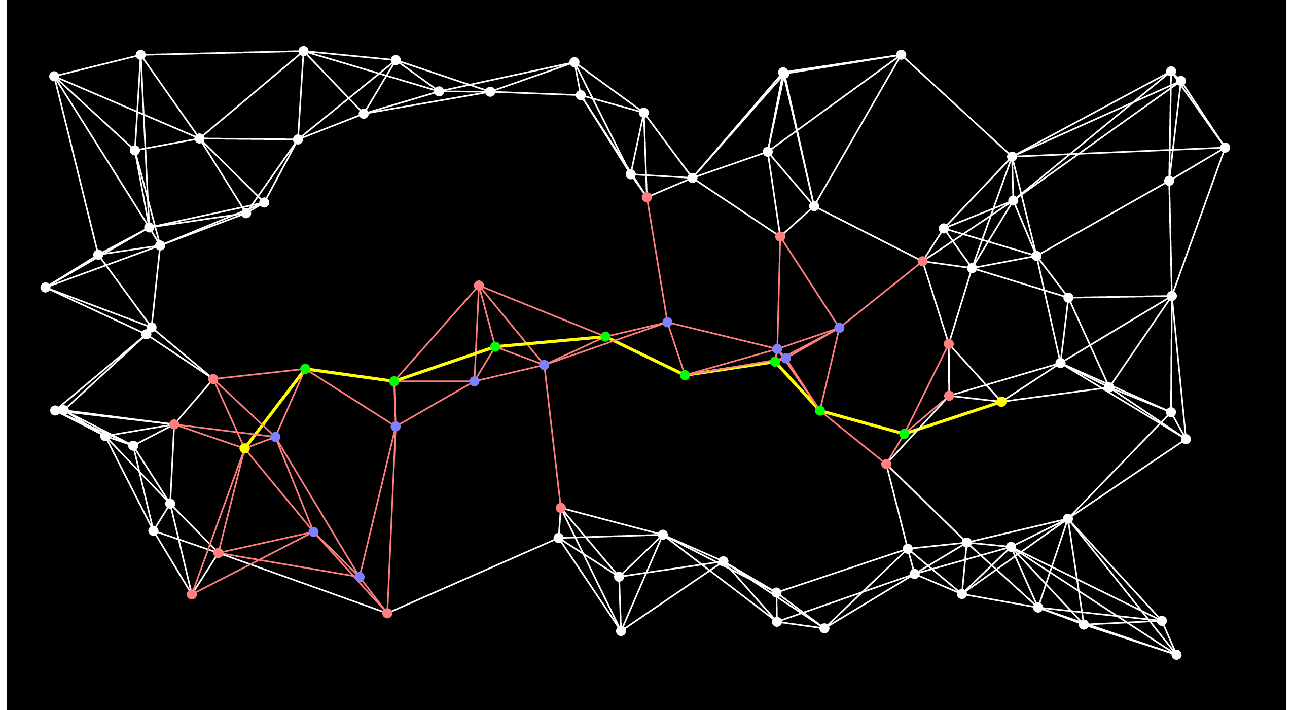
This is the fundamental weakness of Dijkstra's algorithm that A-Star attacks. To hammer it home further, here is Dijstra's algorithm after 50 steps:
 |
You'll note that there are three basic routes through the graph, and Dijkstra's algorithm is considering all of them, because it orders nodes by their distance to Start.
Let's look at A-Star after 50 steps:
 |
It has already found the shortest path! And you'll notice that there are several nodes (e.g. the second one chosen by Dijkstra's algorithm) that never made it out of the open set.
Let's see how A-Star works!
As of this writing, I have taught this lecture 7 times, and I still find these next paragraphs difficult to teach and understand. But I will try, and I will illustrate with an example.
The algorithm works in a very subtle way. With Dijkstra's algorithm, you know when you add a node to the closed set, you know the shortest path to that node. That is not true with A-Star, and that is a little confusing. In fact, with A-Star, you may need to process nodes more than once, so there actually isn't a true "open set" or "closed set". For the moment, though, let's continue to think that way.
With A-Star, consider the actual shortest path, and consider the first node on that path that is in the open set. When you move that node to the closed set, you know the shortest path to that node (because it comes from Start). Moreover, you are guaranteed to move that node to the closed set before you put End into the closed set. Why? Because the distance from Start plus the estimate to End has to be less than any other path to End.
Continuing by induction, you have to put every node on the shortest path into the closed set before you put End into the closed set. This means that when you actually put End into the closed set, you have found its shortest path.
Why do we have this guarantee? Because our estimates are always correct or low.
I won't explain this any further yet. Instead, let me repeat the specification of A-Star in a slightly different way:
What A-Star does to Dijkstra's algorithm is give preference on the multimap to nodes that are likely to belong on the shortest path from Start to End. The cool thing is that when End is the first node in the multimap, you are assured that you have found the shortest path to it!
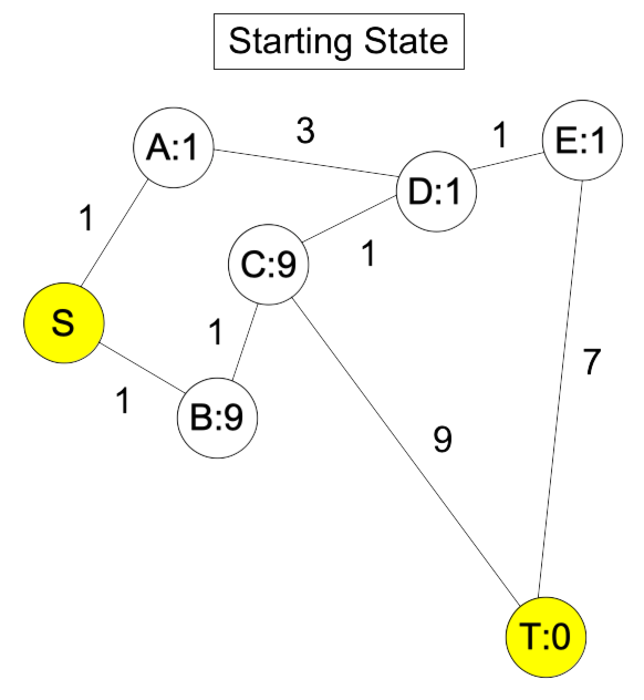
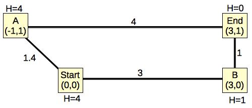
Let's take a really simple example:
 |
The edges are weighted by their Euclidean distances, and I have labeled each node's H value to be its Euclidean distance to End. It should be clear that the actual path length from any node to End will have to be greater than or equal to its H value. In this example, only Start's path length is greater than its H value. The rest are equal.
When you run Dijkstra's algorithm on this graph, you go through the following steps:
Now, let's see how A-Star works.
 Dijkstra |
 A-Star |
As you can see, the difference is the fact that the A node is in the closed set with Dijkstra, but in the open set with A-star. As a result, the edge from A to end was not processed in A-star.
 |
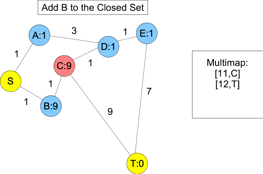
The shortest path is S-B-C-T, but because the estimates for A, D and E are so low, the algorithm guides us to S-A-D-E-T. Here's the graph after we put E into the closed set:
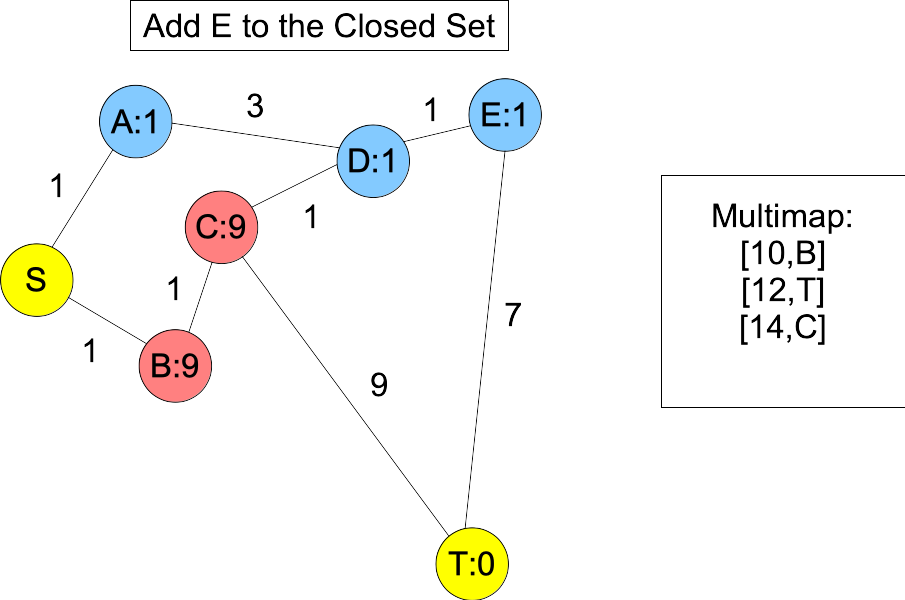 |
You'll note, when we put D and E into the closed set, we don't know the shortest paths to them -- you can get to D with a shorter path: S,B,C,D. However, the next node on the actual shortest path, B, is in the open set and we happen to know its shortest path. Moreover, its distance plus estimate must be less than or equal to the actual shortest path length. Therefore, it will always be in the multimap with a lower value than T. When we add it to the closed set, C becomes the next node on the shortest path in the open set, and you'll note that is is also before T, because its value in the multimap is equal to the actual shortest path length:
 |
You can avoid this by having a consistent heuristic. To be consistent, h() must be such that for every adjacent node X and Y,
In other words, a node's estimate can't be greater than (the distance to any neighbor) + (the neighbor's estimate). This is violated all over the place in the graph above, but the most egregious place is with C and D. C's estimate is 9, which is much bigger than 1+1, which is the distance to D and D's estimate.
Fortunately, in the programs below, I'm using a consistent heuristic, so I can keep the "open set"/"closed set" heuristic.
O -> O -> O -> O -> O -> O -> O -> O | | | | | | | | v v v v v v v v O -> O -> O -> O -> O -> O -> O -> O | | | | | | | | v v v v v v v v O -> O -> O -> O -> O -> O -> O -> O | | | | | | | | v v v v v v v v O -> O -> O -> O -> O -> O -> O -> O | | | | | | | | v v v v v v v v O -> O -> O -> O -> O -> O -> O -> O | | | | | | | | v v v v v v v v O -> O -> O -> O -> O -> O -> O -> O | | | | | | | | v v v v v v v v O -> O -> O -> O -> O -> O -> O -> O |
The reason is that for all nodes on the shortest path, the sum of shortest path from Start and the estimate is equal to the path length from Start to End. So this sum is the same for all nodes that are on any shortest path.
To make A-star effective here, you need to tweak either the algorithm or your estimates here -- the Patel page goes into great length on this, and it's fascinating.
bin/a-star-tester-0 seed xmin ymin xmax ymax nn connections-per-node Dijkstra|A-Star|Nothing print(Y|N|G) |
It will create a random graph on the XY coordinate plane bounded by (xmin,ymin) and (xmax,ymax). The graph will have nn nodes and it will be fully connected. Each node will have roughly connections-per-node edges to nearby nodes. The Start node will be on the left side somewhere, and the End node will be on the right side. When the graph is created, you can then run Dijkstra, A-Star, or nothing on it. At the end, if you specify Y, it will print out the graph using the colors above, using jgraph. If you specify G, it simply prints out a text file representation of the graph before runnning the algorithm. If you specify N, it only prints timing information, and the sizes of the open and closed sets. Finally, if you specify 0 as connections-per-node, it doesn't create the graph, but instead reads its text representation from standard input.
Let's try a simple example:
UNIX> bin/a-star-tester-0 106 -10 -10 10 10 40 5 Nothing G > txt/G-40-5-106.txt
UNIX> bin/a-star-tester-0 106 -10 -10 10 10 40 0 Dijkstra N < txt/G-40-5-106.txt
(* Time:          0.000028 *)
(* Path Length:     12.875 *)
(* Closed Set Size:     25 *)
(* Open   Set Size:     10 *)
(* Unvisited Nodes:      5 *)
UNIX> bin/a-star-tester-0 106 -10 -10 10 10 40 0 A-Star N < txt/G-40-5-106.txt
(* Time:          0.000011 *)
(* Path Length:     12.875 *)
(* Closed Set Size:      7 *)
(* Open   Set Size:     14 *)
(* Unvisited Nodes:     19 *)
UNIX>
If you use the jgraph option (and do a little tweaking, as I am wont to do), you get the following pictures of the above calls:
 Dijkstra |
 A-Star |
The pictures and the output of the programs convey the same thing -- they have both found the same shortest path from Start to the End. However, Dijkstra's algorithm visits more nodes and edges, and has many more nodes in its closed set. A-Star, on the other hand, is much smarter about its closed set, which only has two nodes that aren't on the shortest path.
I'd be remiss if I didn't talk a little about how the program generates its graphs. My intent was to have each node have connections-per-node edges to its closest neighbors. There are some issues with this, of course. First, there is an issue of reflexiveness. Take a look at the rightmost node in the graphs directly above, and suppose that connections-per-node were one instead of five, and suppose that we call the node A, and the one closest to it B. It's pretty clear that A is not the closest node to B, or even one of the four closest nodes to B.
So, what I settled on was the following. I considered the nodes in random order (the order in which they were created). When I considered a node, it may already have had edges on its adjacency list. So, I needed to generate z = (connections-per-node - adjacency.size()) new edges. To do that, I maintained a map of closest nodes, ordered by their distance to the node. It starts empty, and I never let it get bigger than z elements (if it does, I delete the biggest elements on it).
Now, I consider four nodes as candidates for the map:
I can stop when the distance along the given axis is big enough. For example, I can stop considering xlow nodes when the distance between xlow and the node along the x axis is bigger than the largest node in the map.
It's hard to do a formal analysis of this, but it should do a decent job of considering a fairly small subset of the nodes, especially when the number of nodes is large and connections-per-node is small. I would probably do better to break up the grid into squares whose sides are sqrt(|V|) or something like that, and then only look for edges within certain squares. I don't have the time to play with it.
When I'm done with this process, I add the nodes in the map to the node's adjacency list (and add the reverse edges, because these graphs are undirected).
At that point, the graph may be disconnected. To connect it, during the graph generation process, I maintain disjoint sets of connected components. Then, after generated the edges above, I connect the graph by going through the following process -- I choose a random node, and find the closest node to it that is not in the same set. Then, I find the closest node to that one that is not in the same set. The logic there is that the first node that I have chosen may be in the "middle" of its disjoint set. However, the node closest to it will be on the "edge" of its disjoint set. So that's a good node to connect with another disjoint set. That part of the algorithm is O(|V|) for each disjoint set.
I'm left with a fully connected graph, and its running time shouldn't be O(|V|2), which is what I was trying to avoid.
The second program is in src/a-star-tester-2.cpp, which tries to make H better. What it does is the following: When it needs to calculate a node's H value, it doesn't use Euclidean distance. Instead, it considers every node to which it is incident that is not already in the closed set. It calculates the distance to that node, plus that node's Euclidean distance to End, and sets its H value to the minimum of these values. You should see how that gives you H values that are higher than the Euclidean distance, but still less than or equal to the actual shortest path lengh.
If a node is in the open set, and all of its edges are to nodes in the closed set, then there is no way that the node can be on a shortest path. When we discover such a node, we set its H value to ∞.
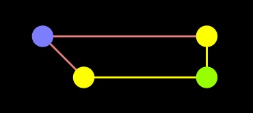
Look at a simple example, which is the first graph I showed you:
 |
Using our new calculation, the Start node's H value is 4, rather than 3.16. That is because Start chose its H value to be the minimum distance-plus-H value to A and B, rather than its Euclidean distance. You should see how that results in a higher, but still legal H value.
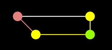
Obviously, the tradeoff in this program is going to be smaller closed-set size, versus more expensive calculation of H. When I first implemented it, here's the picture I got with the above example:
 |
That doesn't look right, does it? The closed set side is bigger than the previous example. The reason is that I used the algorithm to set End's H value, rather than just setting it to zero. That's a bug, and I discovered it by looking at the pictures. I show this just to highlight how important it is to test your programs as you write them!!!. That program is in src/a-star-tester-2.cpp.
The bug is fixed in src/a-star-tester-3.cpp. Here's the output -- you can see that there is one fewer node in the closed set than in the previous A-Star example:
UNIX> bin/a-star-tester-3 106 -10 -10 10 10 40 5 A-Star N < txt/G-40-5-106.txt
(* Time:          0.000008 *)
(* Path Length:     12.875 *)
(* Closed Set Size:      6 *)
(* Open   Set Size:     14 *)
(* Unvisited Nodes:     20 *)
UNIX>
 |
UNIX> bin/a-star-tester-4 106 -10 -10 10 10 40 5 1.1 N < txt/G-40-5-106.txt
(* Time:          0.000011 *)
(* Path Length:     12.875 *)
(* Closed Set Size:      7 *)
(* Open   Set Size:     14 *)
(* Unvisited Nodes:     19 *)
UNIX> bin/a-star-tester-4 106 -10 -10 10 10 40 5 2 N < txt/G-40-5-106.txt
(* Time:          0.000015 *)
(* Path Length:     14.672 *)
(* Closed Set Size:      6 *)
(* Open   Set Size:     15 *)
(* Unvisited Nodes:     19 *)
UNIX>
As you can see, that last call didn't find the shortest path. This is the one that it found. When the factors get really high, the program becomes a greedy DFS using only the Euclidean distances as heuristics, and ignoring the effect of the paths to the nodes.
 |
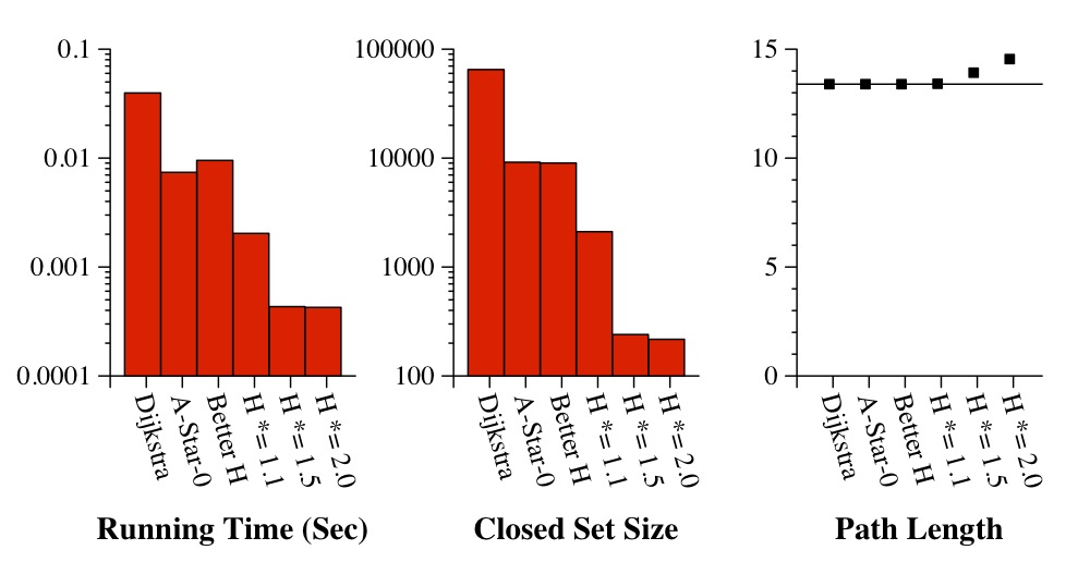
UNIX> bin/a-star-tester-0 1 -10 -10 10 10 10000 3 Nothing G > G-10000-3-1.txtBelow, I show the various programs finding the shortest paths (sometimes):
The graph Finding the yellow nodes is like finding Waldo... |
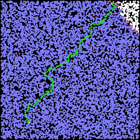 Dijkstra Path Length = 30.706. Time: 0.004342 seconds Closed Set Size: 9729 |
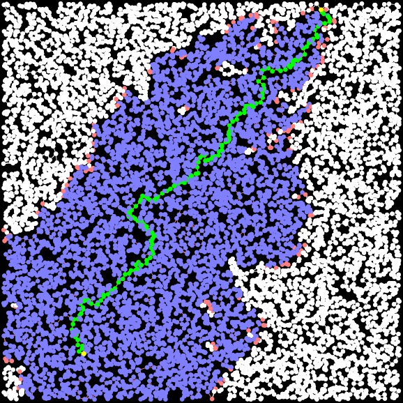 A-Star Path Length: 30.706 Time: 0.002506 seconds Closed Set Size: 4893 |
 A-Star-3 (improved H) Path Length: 30.706 Time: 0.002754 seconds Closed Set Size: 4816 |
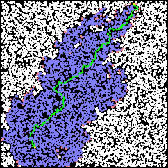 A-Star, Factor = 1.1 Path Length: 30.721 Time: 0.002091 seconds Closed Set Size: 3971 |
 A-Star, Factor = 2 Path Length: 32.212 Time: 0.000481 seconds Closed Set Size: 891 |
A few items of note:
 |
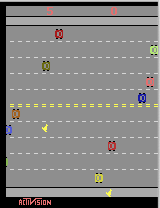 |
In our research, we train spiking neural networks to direct control applications such as video games. In 2020, I needed to learn Python, so I focused on training neural networks for the Freeway application. BTW, if you want to learn about spiking neural networks, please see our group's web site at http://neuromorphic.eecs.utk.edu/. The introductory video -- https://youtu.be/_Ac_PHJyE2Y is four minutes long and does a really nice job of introducing you to spiking neural networks and control applications.
The observations of the Freeway application are brutal -- the old Atari game had 128 bytes of RAM, and that's what you are given. Some research projects use that, and some use the pixel rendering of the game begin played. In our research, we analyzed the RAM to figure out which bytes represented the cars, and which byte represented the Y value of the chicken. We then used these as inputs to training networks.
While working on this, I wanted to know what the "best" performance could be, so I wrote an oracle. The way the oracle works is that it plays the game many times, and each time it plays the came it builds a graph. The nodes of the graph are a combination of the chicken's Y value and the timestep. At each node, you have three choices: up, down and stay. So each node has three edges. The shortest path from (y=0,t=0) to (y=top,t=anything) is the optimal way to play the game with that seed.
There were challenges with this approach. To evaluate each move, I needed to play the game three times. Worse yet, if you arrive at a node in different ways, there's a chance that the same move takes you to a different node. I have an example pictured below:
 |
In this example, "1" means up, "0" means stay, and "2" means down. As you can see, the action out of node (8,14) results in a different edge, depending on how you got to the node. So in my search, I made sure that the same path was always used to get to a node. (You may correctly comment that this means my oracle is not really an oracle. There are only so many hours in the day).
I use A-Star to do the search, and build the graph on the fly. Otherwise, the graph will blow up (it is infinite in size). I didn't try Dijsktra's algorithm, because it would have been too slow, so A-Star was essential. For h(), I simply used the top y value minus the chicken's current y value, divided by the maximum y values that can change on an "up" action. To be honest with you, I'm not sure if that is consistent or not, but it does satisfy the constraint that h() is less than the actual shortest path.
Here's a nice graph from one of the runs:
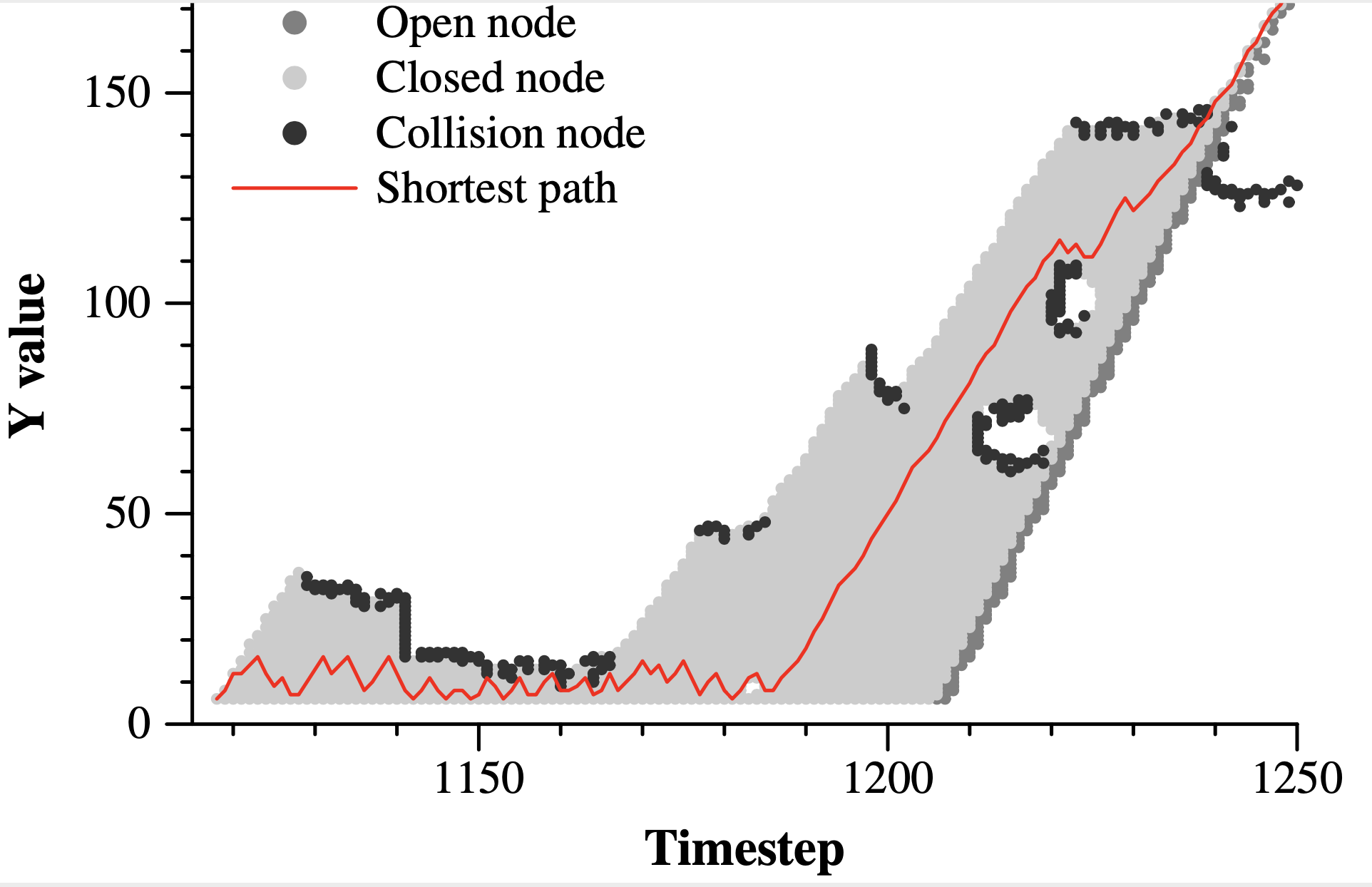 |
You can really see the effectiveness of A-Star here -- imagine how many nodes Dijkstra's algorithm would have!
You can see the results of this activity at https://www.youtube.com/watch?v=FKYXuzNVZKg, where I show 25 perfect runs.
As an aside, in https://www.youtube.com/watch?v=B_nQtRMYVIc, I have a video of one of the spiking neural networks. I call this "the scared chicken", because it is super-cautious. It doesn't score well, but it also avoids collisions very actively. If you care it is a spiking neural network with just two input neurons, three output neurons and two synapses.
The shortest path is the minimum number of moves to get from the current state to the unshuffled state. Like the problem above, you do best to generate the graph on the fly, because it can be huge. The A-Star heuristic of a node is the number of nodes that are in the wrong position.
BTW, a good class presentation would be on problems like this (or from that web site), where you test multiple heuristics for A-Star.