 |
I'll now summarize the algorithm.
I'm not proving here that the Floyd-Warshall algorithm works, by the way. I'm just telling you that it works, and how to do it.
|
You'll note first that it has negative edges. That's ok, as long as there are no negative cycles in the graph (which there aren't). Now, we're going to work through the algorithm, and what I'll do is at each step, show you SP both in graphical form and as a matrix. I'm going to sentinelize the lack of an edge with ∞.
 |
           1     2     3     4
        ----------------------
     1 |   0     ∞    -2     ∞
     2 |   4     0     3     ∞
     3 |   ∞     ∞     0     2
     4 |   ∞    -1     ∞     0
|
Step 1: i = 1. We start with i = 1. We next have to iterate through every pair of nodes (x,y), and test to see if the path from x to y through node i is shorter than SP[x][y]. Obviously, we can ignore the cases when x=i, y=i or x=y. Here are the values that we test: I've colored the "winners" red in each case:
| x | y | SP[x][1] | SP[1][y] | SP[x][1]+SP[1][y] | Old SP[x][y] | New SP[x][y] |
2 2 3 3 4 4 |
3 4 2 4 2 3 |
4 4 ∞ ∞ ∞ ∞ |
-2 ∞ ∞ ∞ ∞ -2 |
2 ∞ ∞ ∞ ∞ ∞ |
3 4 2 4 2 3 |
2 4 2 4 2 3 |
As you can see, there is one place where SP is improved. I'll update the drawing and the matrix below. I've colored the changed edges/values in red, and I colored node 1 in green to show that it was the intermediate node in these paths:
 |
           1     2     3     4
        ----------------------
     1 |   0     ∞    -2     ∞
     2 |   4     0     2     ∞
     3 |   ∞     ∞     0     2
     4 |   ∞    -1     ∞     0
|
Step 2: i = 2. Let's make the same table as before, only now with i = 2:
| x | y | SP[x][2] | SP[2][y] | SP[x][2]+SP[2][y] | Old SP[x][y] | New SP[x][y] |
1 1 3 3 4 4 |
3 4 1 4 1 3 |
∞ ∞ ∞ ∞ -1 -1 |
2 ∞ 4 ∞ 4 2 |
∞ ∞ ∞ ∞ 3 1 |
-2 ∞ ∞ 2 ∞ ∞ |
-2 ∞ ∞ 2 3 1 |
There are two places where SP is improved. I'll update the drawing and the matrix below:
 |
           1     2     3     4
        ----------------------
     1 |   0     ∞    -2     ∞
     2 |   4     0     2     ∞
     3 |   ∞     ∞     0     2
     4 |   3    -1     1     0
|
Step 3: i = 3. Here's our table:
| x | y | SP[x][3] | SP[3][y] | SP[x][3]+SP[3][y] | Old SP[x][y] | New SP[x][y] |
1 1 2 2 4 4 |
2 4 1 4 1 2 |
-2 -2 2 2 1 1 |
∞ 2 ∞ 2 ∞ ∞ |
∞ 0 ∞ 4 ∞ ∞ |
∞ ∞ 4 ∞ 3 -1 |
-2 0 4 4 3 -1 |
Once again there are two places where SP is improved. I'll update the drawing and the matrix below:
 |
           1     2     3     4
        ----------------------
     1 |   0     ∞    -2     0
     2 |   4     0     2     4
     3 |   ∞     ∞     0     2
     4 |   3    -1     1     0
|
The Last Step: i = 4. Here's our table:
| x | y | SP[x][4] | SP[4][y] | SP[x][4]+SP[4][y] | Old SP[x][y] | New SP[x][y] |
1 1 2 2 3 3 |
2 3 1 3 1 2 |
0 0 4 4 2 2 |
-1 1 3 1 3 -1 |
-1 1 7 5 5 1 |
∞ -2 4 2 ∞ ∞ |
-1 -2 4 2 5 1 |
We're done -- the final drawing and matrix are below. As you can see, three values were changed, and there are no more big values on the graph at all.
 |
           1     2     3     4
        ----------------------
     1 |   0    -1    -2     0
     2 |   4     0     2     4
     3 |   5     1     0     2
     4 |   3    -1     1     0
|
The matrix now has your all-pairs shortest paths. If any of the diagonal entries are negative, then your graph has negative cycles, and the matrix is invalid.
I know that was mathy, but we'll give it a practical instance below.
| # | clues | probability | Answer | Comments |
| 0 | { "Y" } |
{ 50 } |
0.5 | Pretty straightforward. One egg. 50% chance of finding it. |
| 1 |
{ "YN",
"NY" } |
{ 100, 50 } |
1.5 | The clues are worthless. 100% chance of egg 0, and 50% chance of egg 1. |
| 2 |
{ "YYY",
  "NYY",
"NNY" } |
{ 100, 0, 0 } |
3.0 | Fred is finding egg 0, and with the clues, will also find eggs 1 and 2 |
| 3 |
{ "NNN",
  "NNN",
"NNN" } |
{ 0, 0, 0 } |
0.0 | Fred's parents are mean. |
| 4 |
{ "NYYNYYNNNN",
  "NNNNYNNNYN",
  "YNNYYYYYNN",
  "YYNYNNNNYN",
  "NYNNNNNNNY",
  "YNYYNNYNNY",
  "NYNNYYYYYY",
  "NYYYYNNNNN",
  "YYNYNNYYYN",
"NNYYNYNYYY"} |
{ 11, 66, 99, 37, 64, 45, 21, 67, 71, 62 } |
9.999891558057332 | I'm not working through this one by hand. |
| 5 |
{ "NNY",
  "NNY",
"NNN" } |
{ 50, 50, 1 } |
1.7525 | I'll go over this one below. |
| 6 |
{ "NY",
"NN" } |
{ 50, 50 } |
1.25 | If you find egg 0 (50%), you'll find egg 1. If you don't find egg 0 (50%), then you have a 50% chance of finding egg 1. The eggspected value is .5*2 + .25*1 = 1.25. |
We are going to define pi to be the probability that you find egg i, either independently or as the result of finding another egg and using clues. Let's use example 6 above to give real numbers to the problem:
First calculate a connectivity matrix named C of zero's and ones: if C[j][i] is equal to one, then egg i is reachable from egg j using clues. Now, you go through the following algorithm to find pi:
Let's now walk through example 5, which is the following graph:
 |
Our connectivity matrix is:
1 0 1
0 1 1
0 0 1
We're going to calculate all of the pi's with one pass through the eggs:
Now, where does Floyd-Warshall come in? You use it to create the connectivity matrix. The clues are a binary relationship, and the connectivity matrix is the transitive closure. So, you start with the adjacency matrix (clues), and then your Floyd-Warshall calculation is the following, which feels too much like Python for my tastes (I'm using variables to match the code below):
For all nodes v:
  For all pairs of nodes i,j:
     If you can't get from node i to node j (i.e. C[i][j] is zero):
       But you can get from i to v and v to j:
         Then set C[i][j] to one, saying you can get from node i to j after all.
I programmed a Floyd-Warshall solution for this in The-Tips-Floyd-If.cpp. Here's the Floyd-Warshall code to calculate C, then the calculation of p, and the calculation of the final return value:
  /* The Floyd-Warshall Calculation -- sorry that I've changed variable names from above: */
  for (v = 0; v < C.size(); v++) {
    for (i = 0; i < C.size(); i++) {
      for (j = 0; j < C.size(); j++) {
        if (!C[i][j] && C[i][v] && C[v][j]) C[i][j] = 1;
      }
    }
  }

  /* Calculate the values of p from the probabilities and reachability: */
  p.resize(C.size(), 0);
  for (i = 0; i < C.size(); i++) {
    x = probability[i];
    x /= 100.0;
    for (j = 0; j < C.size(); j++) {
      if (C[i][j]) p[j] += ((1 - p[j]) * x);
    }
  }

  /* Calculate the final return value */
  x = 0;
  for (i = 0; i < C.size(); i++) x += p[i];

  return x;
}
|
I have also programmed up a solution that uses bit arithmetic instead of the if statement. This solution doesn't do anything fancy with the bits; it simply replaces the if statement with bit arithmetic. This is in The-Tips-Floyd-Bits.cpp. Here's the Floyd-Warshall part:
  for (v = 0; v < C.size(); v++) {
    for (i = 0; i < C.size(); i++) {
      for (j = 0; j < C.size(); j++) {
        C[i][j] |= (C[i][v] & C[v][j]);
      }
    }
  }
|
Think about the tradeoffs with the two pieces of code. With the if statement, you don't evaluate C[i][v] or C[j][v] when C[i][j] is one. That saves some work. On the flip side, if statements involve comparisons and jumps, which require more instructions than the simple bit arithmetic.
Here's the relevant assembly code for each (Intel core i5, compiled with -O2). I find it hard to read, but it does back up the comments above.
if (!C[i][j] && C[i][v] && C[v][j]) C[i][j] = 1; | C[i][j] |= (C[i][v] & C[v][j]); |
One last tweak -- suppose I want to move the c[i][v] lookup out of the inner loop. Why? Because if it's false, I won't have to do the inner loop at all. This is in The-Tips-Floyd-Bits-2.cpp:
  for (v = 0; v < C.size(); v++) {
    for (i = 0; i < C.size(); i++) {
      if (C[i][v]) {
        for (j = 0; j < C.size(); j++) {
          C[i][j] |= C[v][j];
        }
      }
    }
  }
|
Remember this -- it will come in handy for your lab. All of these work on the topcoder examples:
UNIX> for i in 0 1 2 3 4 5 6 ; do         # I'm using bash here
> tip-fw-if $i | tail -n 1
> tip-fw-bits $i | tail -n 1
> tip-fw-bits-2 $i | tail -n 1
> done
0.5000000000
0.5000000000
0.5000000000
1.5000000000
1.5000000000
1.5000000000
3.0000000000
3.0000000000
3.0000000000
0.0000000000
0.0000000000
0.0000000000
9.9998915581
9.9998915581
9.9998915581
1.7525000000
1.7525000000
1.7525000000
1.2500000000
1.2500000000
1.2500000000
UNIX>
I've timed these on my MacBook (2.4 Ghz Core i5), and the results make sense. Because these matrices are dense, C[i][j] is true a lot of the time, and that makes the if statement exit early a lot. On the flip side, C[i][v] is also true a lot, so moving it out of the inner loop doesn't eliminate the inner loop very much.
 |
void DFS::DoDFS(int n, int from)
{
  int j;

  if (visited[n]) return;

  p[n] += ((1 - p[n]) * pr[from]);
  visited[n] = 1;

  for (j = 0; j < Adj[n].size(); j++) {
    DoDFS(Adj[n][j], from);
  }
}
|
  for (j = 0; j < Adj[n].size(); j++) {
    if (!visited[Adj[n][j]]) DoDFS(Adj[n][j], from);
  }
|
The timing results may surprise you:
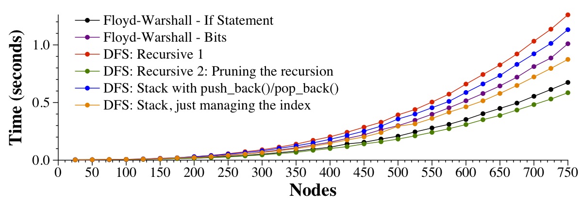 |
They surprise me, as I thought that the stack version with the index would be the best, but instead, it's the pruned recursion. I don't have time to explore it.
  for (v = 0; v < C.size(); v++) {
    for (i = 0; i < C.size(); i++) {
      if (C[i][v]) {
        for (j = 0; j < C.size(); j++) {
          C[i][j] |= C[v][j];
        }
      }
    }
  }
|
Instead of storing one bit per char, what if we packed each char with 8 bits? In other words, we can store an entire row C with ceil(C.size()/8) char's. Let's use an example:
    01234567
   ---------
0 | 10001001
1 | 01100000
2 | 10101000
3 | 00010000
4 | 10001000
5 | 00100100
6 | 00000010
7 | 00100001
In our previous Floyd-Warshall implementations, each entry of the adjacency matrix consumed
a char. What if instead we had each row of the adjacency matrix be a single byte,
and each entry consumes a bit? Look and see what that lets us do in that inner loop.
Suppose v equals 0 and i equals 2. You'll note that C[i][v] equals one.
That means that for each value of j, we will OR C[i][j] with
C[v][j] and set the result in
C[i][j]. Here's row i (2) of C:
2 | 10101000And here's row v (0):
0 | 10001001Since both rows are bytes, we can do the OR in one instruction, which will set row 2 to be:
2 | 10101001Do you see how that can improve performance? Instead of doing 8 OR operations in the inner loop, you only have to do one!
The graph below shows how we use this trick for 1, 2, 4, 8 and 16-byte data types. In that latter case, I'm using the Microsoft Intrinsic instruction _mm_or_si128(), which compiles to code that uses the 128-bit OR instruction from the Intel SSE2 instruction set. Make sure you pay attention to the units on the Y axis -- the savings are HUGE.
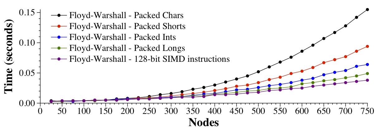 |
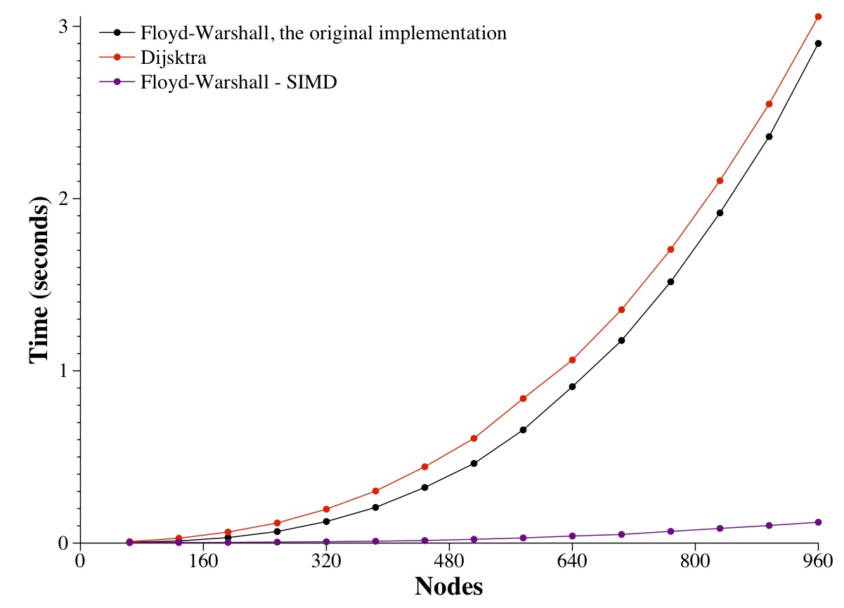
This last graph shows the original Floyd-Warshall implementation, the fastest DFS implementation, and the 128-bit SIMD implementation -- that's an amazing difference, is it not?
 |
An aside for 2017 -- a student, Gregory Rouleau, got a bit enthused pursuing the understanding of performance in The Tips. I'm including his writeups. I love it when students lock into a research question!
The problem that we're going to solve is, given an adjacency matrix of a weighted, directed graph, compute the flow of the maximum flow path between every pair of nodes. We're going to constrain flow values so that they are between 0 and 255. I've drawn an example graph on the left, and its all-pairs max-flow path graph on the right. I've drawn the edges that have been updated with better flow values in red:
 |  |
As you can imagine, we'll solve the problem with the Floyd-Warshall algorithm. To do so, I've written a driver program in AP-Flow-Main.cpp. I have three programs that solve the problem:
usage: AP-Flow nodes seed(- to read from stdin) print(Y|N|H) |
If you give it a seed, it will simply create a random graph. Otherwise, it reads the graph from standard input. If print is "Y", then it will print the graph's adjacency matrix before the flow calculation, and the all-pairs max-flow path matrix after the flow calculation. For example, the graph above was generated with a seed of 12.
UNIX> ap-flow-fw 3 12 Y
Adjacency Matrix:

 255  37  64
  93 255  52
  98  62 255

Flow Matrix:

 255  62  64
  93 255  64
  98  62 255
UNIX>
There is a header file in AP-Flow.h:
class APFlow {
  public:
    int N;
    uint8_t *Adj;
    uint8_t *Flow;
    void CalcFlow();
};
|
N is the number of nodes. Adj is the adjacency matrix, where Adj[i*N+j] stores the weight of the edge from i to j. Flow will be the flow matrix. You will create it by calling CalcFlow(). When CalcFlow() finishes then Flow[i*N+j] will contain the flow of the maximum flow path from i to j. AP-Flow-Main.cpp creates an instance of the class, and initializes N and Adj. It then calls CalcFlow(). If print is 'Y', then it prints out the two matrices. If print is 'H', then it prints out the MD5 hash of Flow. That allows us to check correctness without having to look at giant matrices:
UNIX> ap-flow-fw 5 1 Y
Adjacency Matrix:

 255   8  41  52  19
  44 255   1  11   5
  27  44 255  49  60
  29  12 108 255 115
  53  29  11  29 255

Flow Matrix:

 255  44  52  52  52
  44 255  44  44  44
  53  44 255  52  60
  53  44 108 255 115
  53  44  52  52 255
UNIX> ap-flow-fw 5 1 H
3B65A77BC185B3A15603EF2268873233
UNIX> ap-flow-d 5 1 H
3B65A77BC185B3A15603EF2268873233
UNIX>
BTW, the diagonal elements are always given a weight of 255.
The Floyd-Warshall solution in AP-Flow-FW.cpp is straightforward, and is very much like our other Floyd-Warshall solutions. What we're doing now, is saying that if the path from i to j through v has a higher flow value than what we currently know (which is in Flow[i*N+j]), then update it:
#include "AP-Flow.h"

void APFlow::CalcFlow()
{
  int i, j, v, f;

  for (i = 0; i < N*N; i++) Flow[i] = Adj[i];

  for (v = 0; v < N; v++) {
    for (i = 0; i < N; i++) {
      for (j = 0; j < N; j++) {
        /* f is the flow from i to j through v */
        f = (Flow[i*N+v] < Flow[v*N+j]) ? Flow[i*N+v] : Flow[v*N+j];
        if (f > Flow[i*N+j]) Flow[i*N+j] = f;
      }
    }
  }
}
|
I won't go through the Dijkstra solution, but suffice it to say that it is slower than Floyd-Warshall:
UNIX> sh
sh-3.2$ for i in 160 320 480 960 ; do csh -c "time ap-flow-fw $i 1 N"; done
0.016u 0.000s 0:00.01 100.0%	0+0k 0+0io 0pf+0w
0.118u 0.000s 0:00.12 91.6%	0+0k 0+0io 0pf+0w
0.381u 0.001s 0:00.38 100.0%	0+0k 0+0io 0pf+0w
2.905u 0.004s 0:02.91 99.6%	0+0k 0+0io 0pf+0w
sh-3.2$ for i in 160 320 480 960 ; do csh -c "time ap-flow-d $i 1 N"; done
0.039u 0.000s 0:00.04 75.0%	0+0k 0+0io 0pf+0w
0.193u 0.000s 0:00.19 100.0%	0+0k 0+0io 0pf+0w
0.516u 0.001s 0:00.51 100.0%	0+0k 0+0io 0pf+0w
3.036u 0.004s 0:03.04 99.6%	0+0k 0+0io 0pf+0w
sh-3.2$ exit
UNIX>
Now, as with the connectivity problem above, we can use SIMD to make this faster. I'm going to illustrate by annotating the Floyd-Warshall solution:
#include "AP-Flow.h"

void APFlow::CalcFlow()
{
  int i, j, v, f;

  for (i = 0; i < N*N; i++) Flow[i] = Adj[i];

  for (v = 0; v < N; v++) {
    for (i = 0; i < N; i++) {

      /* Create a vector alli, which is 16 instances of Flow[i*N+v] */

      for (j = 0; j < N; j += 16) {

        /* Load Flow[v*N+j] through Flow[v*N+j+15] to vector vv */

        /* Create fv, which is the flow from i to each of j through j+15
           through v. This is simply the min of alli and vv. */

        /* Load Flow[i*N+j] through Flow[i*N+j+15] to vector iv */

        /* Create rv, which is the max of each value of fv and iv. */

        /* Store rv into Flow[i*N+j] through Flow[i*N+j+15] */
      }
    }
  }
}
|
Let me illustrate. Suppose that N is 16, and suppose that row i is:
30 95 101 255 104 106 69 106 11 109 73 75 108 7 15 37Let's suppose that v is 2, and let's also suppose that row v is:
119 66 255 62 80 4 47 123 48 99 22 35 100 31 13 99Now, the flow from i to v is 101. The current flow from i to 0 is 30. However, I can get from i to v with a flow of 101, and from v to 0 with a flow of 119. That means that I can get from i to 0 through v with a flow of 101, and I should update entry zero in row i to be 101.
On the flip side, the flow from i to 1 is 95, and the flow from v to 1 is 66, so I can't improve my flow by going through v.
This should give you a flavor of how row i gets updated using the flow from i to v and row v. Now, let's do it with SIMD:
alli     101 101 101 101 101 101 101 101 101 101 101 101 101 101 101 101
vv       119  66 255  62  80   4  47 123  48  99  22  35 100  31  13  99
fv       101  66 101  62  80   4  47 101  48  99  22  35 100  31  13  99
iv        30  95 101 255 104 106  69 106  11 109  73  75 108   7  15  37
rv       101  95 101 255 104 106  69 106  48 109  73  75 108  31  15  99
You'll store rv as the new value of row i.
That is your job -- to write AP-Flow-SIMD.cpp, which solves the all-pairs max-flow paths problem using Floyd-Warshall and SIMD. You may assume that N is always a multiple of 16. My program simply exits if it is not:
UNIX> ap-flow-simd 17 1 H
For SIMD, N must be a multiple of 16
UNIX>
The only SIMD routines that you need to solve this problem are _mm_set1_epi8(), _mm_min_epu8() and _mm_max_epu8().
How much faster is this? Oh my.....
 |