Project 6 - Particle Swarm Optimization

Project 6 — Particle Swarm Optimization

Parameters

The following is some guidance for the ranges of the parameters.

Number of particles: A typical range is 20-40. For many problems, as few as 10 particles may be enough. For larger or more difficult problems, 100, 200, or more particles might be more appropriate.

Inertia: Generally the range is 0-1, typically very close to 1.

Cognition and social parameters: Usually they are nearly equal and typically around 2, but they can range from 0-4.

World width and world height: The range in the x and y directions, respectively. A good range is -50 to 50 in both directions. In that case, both the world width and height would be 100.

Maximum velocity: Limits how much a particle can move for a given iteration. Typical values to try are 1, 2, and 10. Some implementations define maximum velocity as the world width or height.

Data representation

It's probably easiest to keep the x and y coordinates in separate arrays/variables for position, velocity, personal best, and global best.

Initialization

The position of each particle should be initialized to a random number in the range for each coordinate (e.g. between -50 and 50 in both directions).

The velocity of each particle can be initialized to 0.

The personal best for each particle can be initialized to that particle.

The global best can be initialized to the particle with the best fitness, as given by the objective functions Q(p) (i.e. Q(position)).

Of course, both the x and y coordinates of each of these should be initialized.

Stopping condition for main update loop

Keep iterating until the error in the x and y coordinates drops below a certain threshold (e.g. 0.01). In case the system never fully converges, a second condition should be added, which is a maximum number of iterations. Both of these conditions can be given in a while loop.

Updating the particles

Implement the following update rules:

Velocity

 velocity' = inertia * velocity + c_1 * r_1 *
      (personal_best_position - position) + c_2 * r_2 *
      (global_best_position - position)

where c_1 is the cognition parameter, c_2 is the social parameter, and r_1 and r_2 are random numbers from 0-1.

The positions and velocities are actually vectors, so you would implement this formula for both the x and the y coordinates.

The velocity needs to be scaled in order to keep it within range. Otherwise, the positions will become too large and often go out of bounds, and your program will behave wildly. The following is how to scale the velocity:

 if abs(velocity) > maximum_velocity² 

        velocity = (maximum_velocity/sqrt(velocity_x²
      + velocity_y²)) * velocity

Again, do this for both the x and y coordinates.

Position

position' = position + velocity'

Personal best

 if(Q(position) > Q(personal_best_position)) 

        personal_best_position = position

Global best

 if(Q(position) > Q(global_best_position)) 

        global_best_position = position

Measuring performance

At the very least, calculate the average error in the x and y coordinates of the particles. This can be done by

 error_x += (position_x[k] - global_best_position_x)²
      

      error_y += (position_y[k] - global_best_position_y)²

for each particle k.

Then

 error_x = sqrt((1/(2*num_particles))*error_x) 

      error_y = sqrt((1/(2*num_particles))*error_y)

This is the measure that should be included as part of your stopping condition.

You can plot this error over the number of iterations to get a qualitative view of the performance.

As mentioned in the Project 6 handout, you can also compute the percentage of particles that have converged to within a small distance of the global maximum. You can also plot this over the number of iterations.

Number of epochs until convergence is another measure of performance.

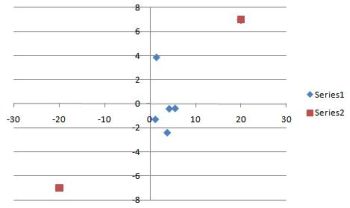
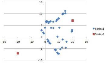
A purely qualitative assessment is to obtain a scatter plot of the particles after the updating iterations. Below are two examples of what you might see for Problem 2 (two maxima). In the first graph, most of the points have converged to the global maximum, although they are covered up by the global maximum point on the graph.

The more performance measures and graphs you analyze, the higher grade you can earn.

Neighborhood (local) best (COSC 427/527 part)

The requirement is to implement a ring topology with neighborhoods given by the 2-nearest neighbors. Define a permutation of the particles, where a particle's neighbors are the array elements before and after it (allow for wraparound). You can use the position arrays as the permutation, where the neighbors are accessed by the array indices. The topology will not change during the iterations of the algorithm. That is, each particle will keep its same two neighbors throughout the iterations.

The velocity formula is modified as follows:

 velocity' = inertia * velocity + c_1 * r_1 *
      (personal_best_position - position) + c_2 * r_2 *
      (global_best_position - position) + c_3 * r_3 *
      (local_best_position - position)

The best neighbor is the particle whose Q(position) is the largest.

You can try k-nearest neighbors for extra credit. For example, 4-nearest neighbors are given by the 2 elements before and the 2 elements after the given particle.

For the Euclidean distance method (extra credit), the nearest neighbors of a particle are those that are within a given radius as measured by Euclidean distance. The radius is another parameter that can vary over a range of values.

You can also try other topologies for extra credit, such as star or wheel.