 |
There is more material in the following Wikipedia pages. As with a lot of Wikipedia, the presentation is too dry and mathematical, so I don't require that you read it, but I provide links to it anyway:
There are two special nodes, called the source and the sink You assume that there is an infinite source of water at the source. The Network Flow problem is as follows: What is the maximum volume of water that can flow from the source to the sink per unit time? No edge can hold more flow than its capacity, and the amount of flow going into a node has to equal the amount of flow going out of a node.
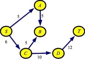
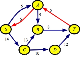
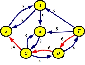
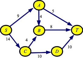
Here's an example graph, with source S and sink T (in this and other pictures, you can click on the pictures, and get the full size picture):
|
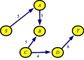
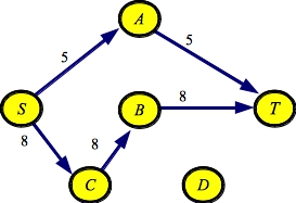
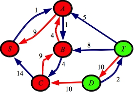
It's not hard to eyeball this graph, and determine that the maximum flow is 23. Here's a graph that shows this flow, subject to the above rules:
 |
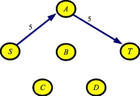
Let's try this on the example above. Below, I'll show three pictures: The first removes five units of flow from the path S-A-T, then eight units of flow from the path S-C-B-T, and finally six units of flow from the path S-C-D-T:
| Remove 5 units of flow from S-A-T:
|
Remove 8 units of flow from S-C-B-T:
|
Remove 6 units of flow from S-C-D-T:
|
You'll note that the source is no longer connected to the sink, so we can't find any more paths with flow. But we've only found 19 units of flow, and not 23. In other words, our algorithm doesn't work.
Let's go back to our example above. Below is the starting state of the flow graph and the residual graph:
| Flow Graph
|
Residual Graph
|
Like before, we start with the path S-A-T. It has a flow of 5. So, we'll add that path to the flow graph, subtract the flow from S-A-T, and also add ``reverse'' flow along the path T-A-S. Here is the result. I'm drawing the ``reverse'' flow in red, since this flow is usually the one that confuses students.
| Flow Graph
|
Residual Graph
|
Also like before, let's choose our next path to be S-C-B-T, with a flow of 8. We'll add it to the flow graph, subtract it from the residual, and add the reverse flow to the residual:
| Flow Graph
|
Residual Graph
|
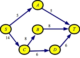
Also like before, let's choose our third path to be S-C-D-T, with a flow of 6. We'll add it to the flow graph, subtract it from the residual, and add the reverse flow to the residual:
| Flow Graph
|
Residual Graph
|
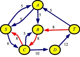
You'll recall that this is the point at which we were stuck above. However, the reverse edges have now given us another path through the graph: S-A-B-C-D-T, with a flow of four. Let's process those:
| Flow Graph
|
Residual Graph
|
Now, there's no way to get from the source to the sink in the residual graph. Therefore, our final network flow is 23 units.
Again, we call this the ``Ford-Fulkerson'' algorithm. You'll note that it does not specify how we find the augmenting paths. That will be an important problem that we will address later.
| Residual Graph
|
Original Graph
|
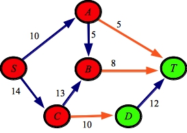
The minimum cut is composed of all edges in the original graph, from the red set to the green set. These are highlighted in orange above: AT, BT and CD.
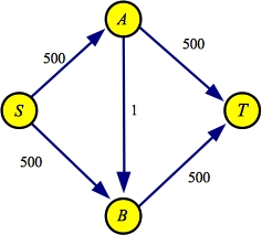 |
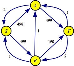
It's pretty easy to eyeball this graph and see that it has a maximum flow of 1000. The two paths are S->A->T and S->B->T. However, if you try to determine the maximum flow using augmenting paths, and you choose the wrong path at each step, it will take 1000 iterations of the algorithm. To illustrate, suppose that the first path you choose is S->A->B->T with a flow of one. When you process this path through the residual graph, you end up with the following:
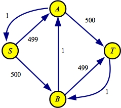 |
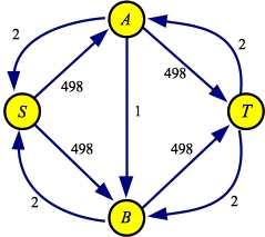
At the next iteration, suppose you choose the path S->B->A->T, again with a flow of one. The residual looks as follows:
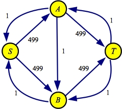 |
You continue in that vein. The pictures below show how you choose S->A->B->T again, and then S->B->A->T, again:
 |  |
Each time, you add one unit of flow, which means that this will take 1000 iterations. Although this example is unlikely to happen in practice, it demonstrates a need for a smart determination of paths.
Now, a matching of a graph is a collection of edges where no two edges share a node. A classic problem from graph theory is given a bipartite graph, determine a matching that has maximum size. You'll note, this is the problem that your network flow lab solves.
You can use network flow to determine the maximum matching of a bipartite graph. You do that by adding two nodes to your graph -- a source S and a sink T. You add an edge from the source to every node in the first set, and an edge from every node in the second set to the sink. And you set the capacity of all edges to one. Now, determine the maximum flow of the graph. In the flow graph, any edge going from one set to the other is part of the matching.
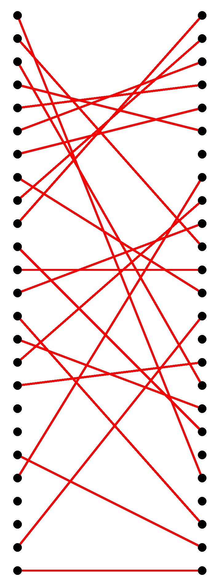
Here's a pretty beefy example. Below is a bipartite graph, where all of the nodes in one set are on the left, and all of the nodes in the other set are on the right. To the right is the graph that we construct for network flow -- the source is on the left and the sink is on the right:
 |
 |
When we run network flow on it, we get the flow graph on the left, and if we just isolate the red edges that go from one set to the other, we get the maximum matching:
 |
 |
You can prove to yourself all of the components here: