CS302 Lecture Notes - Breadth First Search and Dikjstra's Algorithm
- James S. Plank
- November 2, 2009.
Latest Modification:
Sat Feb 16 09:01:14 EDT 2019 (by SJE)
- Directory: /home/plank/cs302/Notes/BFS
Reference Material Online
Topcoder Practice Problems
- BFS: The
Topcoder "CarrotJumping" problem (SRM 478, D1, 250).
- BFS:
The Topcoder "EmoticonsDiv1" problem (SRM 612, D1, 250. This link has an
explanation of the BFS and commented code. This problem is similar in flavor to
"CarrotJumping," because you build the graph as you go.
-
BFS:
The Topcoder "StepsConstruct" problem (SRM 707, D2, 500). Dr.
Plank give's you hints and programming tips. There is a commented solution
at the end.
- BFS: The
Topcoder "OneRegister" problem (SRM 486, D1, 250). Dr. Plank
gives hints here too, no code.
- BFS: CollectingRiders (SRM 382, D1, 250). Hints and no code.
- BFS: FromToDivisible (SRM 699, D1, 500). Hints and no code.
- Dijkstra: ColorfulRoad (SRM 596, D2, 500). Hints and no code.
- Dijkstra: The
Topcoder "ThreeTeleports" problem (SRM 519, D2, 600). Hints here, no code.
- Dijkstra: InsertSort (SRM 351, D2, 1000-pointer). Hints and no code.
Breadth First Search (BFS) is complementary to Depth First Search (DFS).
DFS works by visiting a node and then recursively visiting children.
You can view it as relying on a stack -- push a node onto a stack,
then go through the following algorithm:
- Pop a node off the stack.
- Do some processing on the node.
- Push all of the node's children onto the stack.
- Repeat until the stack is empty.
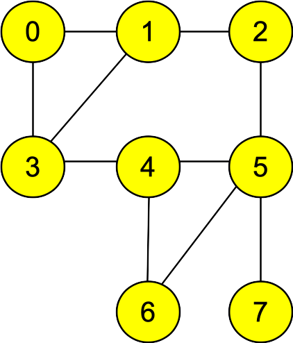
In fact, it will be useful to revisit DFS with this view. Let's use the following
graph as an example:
Adjacency Lists:
 0: 1, 3
 1: 0, 2, 3
 2: 1, 5
 3: 0, 1, 4
 4: 3, 5, 6
 5: 4, 6, 7
 6: 4, 5
 7: 5
|
 |
A recursive visiting of all nodes using DFS starting with node zero will
look as follows:
Were we to print out the nodes, they would be printed out in the order in which they are visited:
0, 2, 9, 8, 10, 3, 7, 6, 4, 11, 1, 5
Instead of recursion, let's use a stack. We'll push 0 onto the stack, then repeatedly
pop a node off the stack, visit the node, then push the non-visited children onto the stack.
(We push the children onto the stack in reverse order so that the order of visiting is the
same as the recursive case).
               Visited?
Node   Print   01234567   Action          Stack (Push-back and pop-back)
               --------   Push 0          0
0      0       x-------   Push 3, 1       3, 1
1      1       xx------   Push 3, 2       3, 3, 2
2      2       xxx-----   Push 5          3, 3, 5
5      5       xxx--x--   Push 7, 6, 4    3, 3, 7, 6, 4
4      4       xxx-xx--   Push 6, 3       3, 3, 7, 6, 6, 3
3      3       xxxxxx--   No pushing      3, 3, 7, 6, 6
6      6       xxxxxxx-   No pushing      3, 3, 7, 6
6              xxxxxxx-   Visited         3, 3, 7
7      7       xxxxxxxx   No pushing      3, 3
3              xxxxxxxx   Visited         3
3              xxxxxxxx   Visited
                          Done
|
As you see, the order of the nodes is the same as in the recursive case.
Now, breadth-first search works in the same manner, only we use a queue instead of a stack.
See how this differs:
Node Visited
0
2
11
9
1
4
8
3
8
6
10
3
6
7
5
7
| Action
Start
Append 2 and 11
Append 9
Append 1 and 4
Append 8 and 3
Do nothing
Append 8 and 6
Append 10, 3 and 6
Append 7
Already visited
Append 5, and 7
Do nothing
Already visited
Already visited
Do nothing
Do nothing
Already visited
| Queue
0
2, 11
11, 9
9, 1, 4
1, 4, 8, 3
4, 8, 3
8, 3, 8, 6
3, 8, 6, 10, 3, 6
8, 6, 10, 3, 6, 7
6, 10, 3, 6, 7
10, 3, 6, 7, 5, 7
3, 6, 7, 5, 7
6, 7, 5, 7
7, 5, 7
5, 7
7
| Print
0
2
11
9
1
4
8
3
6
10
7
5
|
The order of the nodes is now 0, 2, 11, 9, 1, 4, 8, 3, 6, 10, 7, 5.
The algorithm still visits all nodes and edges, but it does so in order of distance from the starting node.
Think about it.
- The first two nodes visited are those that are one edge from node 0: nodes 2 and 11.
- Next are the nodes that are two edges away: nodes 9, 1 and 4.
- Next are the nodes that are three edges away: nodes 8, 3 and 6.
- Finally come the nodes that are four edges away: 10, 7 and 5.
Thus, breadth-first search is a convenient way to find the shortest path from a starting node to
all the other nodes in the graph. To do so, you can store a back-edge in each node n -- this
is the edge that first put n onto the queue. You can also maintain node n's distance to
the starting node. The BFS algorithm becomes:
- For all nodes, set their backedges to NULL and their distances to -1.
- Set node 0's distance to zero and put it on the queue.
- Repeat the following:
- Remove a node n from the queue.
- For each edge e from n to n2 such that n2's distance is -1:
- Set n2's distance to n's distance plus one.
- Set n2's backedge to e.
- Append n2 to the queue.
When the algorithm terminates, each node contains its shortest distance to node zero, and the
path to node zero can be obtained by traversing the backedges.
Once the BFS finishes, we know the shortest distance of every node from node zero, and we can use
the backedges to find the paths. For example, the shortest path from node 0 to node 7 is:
(0,2)(2,9)(9,3)(3,7)
Dijkstra's Algorithm
Dijkstra's algorithm is a simple modification to breadth first search. It is used to find the
shortest path from a given node to all other nodes, where edges may have non-negative weights.
The modification uses a multimap instead of the queue. The multimap uses the distance to
from the starting node to the node as a key, and the node itself as a val.
The algorithm is as follows:
- For all nodes, set their backedges to NULL, their distances to -1, and their "visited"
field to be false.
- Set node 0's distance to zero and put it on the multimap.
- Repeat the following:
- Remove a node n from the front of the multimap and set its visited field to true.
- For each edge e from n to n2 such that n2 has not been visited.
Let d be n's distance plus the weight of edge e.
If n2's distance is -1, or if d is less than node n2's current distance:
- If n2 was in the multimap, remove it. [* We're going to revisit this below. *]
- Set n2's distance to d.
- Set n2's backedge to e.
- Insert n2 into the multimap, keyed on distance.
When the algorithm terminates, all the nodes will contain their shortest distance to node 0,
and their backedges will define the shortest paths.
[* Revisiting Here *]: You actually have a choice of whether to remove a node from the multimap
or not. It is often easier to code up Dijkstra's algorithm to leave nodes on the multimap
rather than remove them. In that case, when a node reaches the front of the multimap for
you to process, you need to check its distance versus its key in the multimap.
If they
differ, you simply ignore the node, because you have processed it already.
The tradeoff
is memory and potentially performance vs coding complexity. When you code, it is much
easier to leave the node on the multimap. However, if you end up replacing a lot of nodes
on the multimap, it can make performance and memory consumption suffer. Ideally, it is
better to remove the node before you re-insert it. To do that properly, you need to store
an iterator to the node's place in the multiple, in the node's class definition. Think
about that, especially if you decide to remove the node in your own implementation. BTW,
I do advocate that you try removing the node in your lab. Not only is the code better,
but it forces you to think about data structure design..
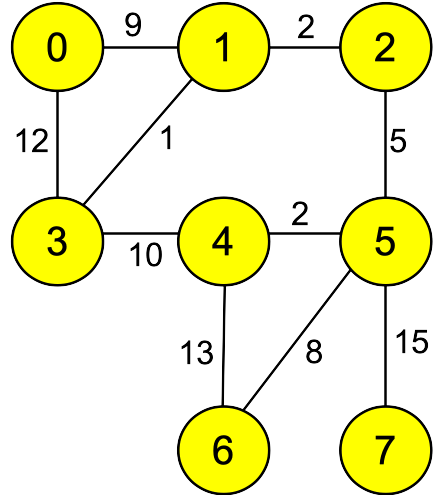
As an example, suppose we enrich the graph above with edge weights:
As with the BFS run above, you can use the backedges to find the shortest paths. For example,
the shortest path from node 0 to node 3 has a distance of 20, and contains the edges:
(0,11)(11,4)(4,8)(8,9)(9,3)
Running Times
The running time of BFS (and therefore the unweighted shortest path problem) is O(|V| + |E|).
As with DFS, it visits each node and edge once.
The running time of Dijkstra's algorithm (and therefore the weighted shortest path problem)
is a little more complex: O(|V| + |E|log(|V|)).
This is because Dijkstra's algorithm visits each node and edge once,
and at each edge, it potentially inserts a node into the multimap.
Memorize those running times!


