 |
Merge sort works with an ingenious recursion, which Dr. Plank outlines as follows:
8.70 7.50 7.86 3.69 9.22 0.96 6.92 1.71The first thing that we do is split this into two 4-element vectors. Dr. Plank colors one light red and one light blue:
Part 1                        Part 2
8.70 7.50 7.86 3.69           9.22 0.96 6.92 1.71
Now, we sort the vectors recursively, which is sort of a leap of faith, but that's how recursion works. When we're done, here's what they look like:
Part 1                        Part 2
3.69 7.50 7.86 8.70           0.96 1.71 6.92 9.22
Now, we want to merge them together into one sorted vector. One thing we know -- the first element of the sorted vector will be either the first element of the light red vector, or the first element of the light blue vector. It will be the smaller of the two -- in this case, 0.96. So, we copy that value to our final vector, and concentrate on the second value from the light blue vector:
Part 1                        Part 2                        Final Vector
3.69 7.50 7.86 8.70           0.96 1.71 6.92 9.22           0.96
Now, we're comparing 3.69 from the red vector, and 1.71 from the blue vector -- we copy the smallest of these, 1.71, to the final vector, and concentrate on the next value in the blue vector:
Part 1                        Part 2                        Final Vector
3.69 7.50 7.86 8.70           0.96 1.71 6.92 9.22           0.96 1.71
Next, we compare 3.69 from the red vector, and 6.92 from the blue vector -- again, we copy the smallest of these, 3.69, to the final vector, and concentrate on the next value in the red vector:
Part 1                        Part 2                        Final Vector
3.69 7.50 7.86 8.70           0.96 1.71 6.92 9.22           0.96 1.71 3.69
By now, you probably see how it will finish -- Here are the last five steps:
Part 1                        Part 2                        Final Vector
3.69 7.50 7.86 8.70           0.96 1.71 6.92 9.22           0.96 1.71 3.69 6.92
3.69 7.50 7.86 8.70           0.96 1.71 6.92 9.22           0.96 1.71 3.69 6.92 7.50
3.69 7.50 7.86 8.70           0.96 1.71 6.92 9.22           0.96 1.71 3.69 6.92 7.50 7.86
3.69 7.50 7.86 8.70           0.96 1.71 6.92 9.22           0.96 1.71 3.69 6.92 7.50 7.86 8.70
3.69 7.50 7.86 8.70           0.96 1.71 6.92 9.22           0.96 1.71 3.69 6.92 7.50 7.86 8.70 9.22
As it turns out, merging is a linear operation -- O(n) in the size of the vector. We'll talk about the overall running time of merge sort later. For now, let's think about implementation. Here's what Dr. Plank suggests that you use as your recursive call. It will be slightly different for the group project:
| void recursive_sort(vector <double> &v, vector <double> &temp, int start, int size, int print); |
The original vector is v, and temp is a temporary vector. Both are the same size. Recursive_sort() will only sort the elements from start to start+size. If size is equal to 1, then it simply returns. If size equals 2, then it sorts the elements directly. Otherwise, It calls recursive_sort() on the first size/2 elements, and on the last size-size/2 elements. When that's done, it merges them into temp, and then copies the elements in temp back to v. It is an unfortunate fact with merge sort that we need a temporary vector.
Let's take a quick look at the output of merge_1_sort. Whenever recursive_sort() is called with a size greater than one, it prints out "B:", start and size (both padded to 5 characters) and the vector. Right before a call to recursive_sort() returns, it does the same thing, only it prints "E" instead of "B". Below is an example of sorting 16 elements. I'm coloring the elements on which each call is focused in light red when recursive_sort() is first called ("B"), and yellow right when recursive_sort() is about to return ("E"):
UNIX> ./merge_1_sort 16
B:     0    16        0.42  4.54  8.35  3.36  5.65  0.02  1.88  9.90  7.50  3.66  3.51  5.73  1.33  0.64  9.51  1.54
B:     0     8        0.42  4.54  8.35  3.36  5.65  0.02  1.88  9.90  7.50  3.66  3.51  5.73  1.33  0.64  9.51  1.54
B:     0     4        0.42  4.54  8.35  3.36  5.65  0.02  1.88  9.90  7.50  3.66  3.51  5.73  1.33  0.64  9.51  1.54
B:     0     2        0.42  4.54  8.35  3.36  5.65  0.02  1.88  9.90  7.50  3.66  3.51  5.73  1.33  0.64  9.51  1.54
E:     0     2        0.42  4.54  8.35  3.36  5.65  0.02  1.88  9.90  7.50  3.66  3.51  5.73  1.33  0.64  9.51  1.54
B:     2     2        0.42  4.54  8.35  3.36  5.65  0.02  1.88  9.90  7.50  3.66  3.51  5.73  1.33  0.64  9.51  1.54
E:     2     2        0.42  4.54  3.36  8.35  5.65  0.02  1.88  9.90  7.50  3.66  3.51  5.73  1.33  0.64  9.51  1.54
E:     0     4        0.42  3.36  4.54  8.35  5.65  0.02  1.88  9.90  7.50  3.66  3.51  5.73  1.33  0.64  9.51  1.54
B:     4     4        0.42  3.36  4.54  8.35  5.65  0.02  1.88  9.90  7.50  3.66  3.51  5.73  1.33  0.64  9.51  1.54
B:     4     2        0.42  3.36  4.54  8.35  5.65  0.02  1.88  9.90  7.50  3.66  3.51  5.73  1.33  0.64  9.51  1.54
E:     4     2        0.42  3.36  4.54  8.35  0.02  5.65  1.88  9.90  7.50  3.66  3.51  5.73  1.33  0.64  9.51  1.54
B:     6     2        0.42  3.36  4.54  8.35  0.02  5.65  1.88  9.90  7.50  3.66  3.51  5.73  1.33  0.64  9.51  1.54
E:     6     2        0.42  3.36  4.54  8.35  0.02  5.65  1.88  9.90  7.50  3.66  3.51  5.73  1.33  0.64  9.51  1.54
E:     4     4        0.42  3.36  4.54  8.35  0.02  1.88  5.65  9.90  7.50  3.66  3.51  5.73  1.33  0.64  9.51  1.54
E:     0     8        0.02  0.42  1.88  3.36  4.54  5.65  8.35  9.90  7.50  3.66  3.51  5.73  1.33  0.64  9.51  1.54
B:     8     8        0.02  0.42  1.88  3.36  4.54  5.65  8.35  9.90  7.50  3.66  3.51  5.73  1.33  0.64  9.51  1.54
B:     8     4        0.02  0.42  1.88  3.36  4.54  5.65  8.35  9.90  7.50  3.66  3.51  5.73  1.33  0.64  9.51  1.54
B:     8     2        0.02  0.42  1.88  3.36  4.54  5.65  8.35  9.90  7.50  3.66  3.51  5.73  1.33  0.64  9.51  1.54
E:     8     2        0.02  0.42  1.88  3.36  4.54  5.65  8.35  9.90  3.66  7.50  3.51  5.73  1.33  0.64  9.51  1.54
B:    10     2        0.02  0.42  1.88  3.36  4.54  5.65  8.35  9.90  3.66  7.50  3.51  5.73  1.33  0.64  9.51  1.54
E:    10     2        0.02  0.42  1.88  3.36  4.54  5.65  8.35  9.90  3.66  7.50  3.51  5.73  1.33  0.64  9.51  1.54
E:     8     4        0.02  0.42  1.88  3.36  4.54  5.65  8.35  9.90  3.51  3.66  5.73  7.50  1.33  0.64  9.51  1.54
B:    12     4        0.02  0.42  1.88  3.36  4.54  5.65  8.35  9.90  3.51  3.66  5.73  7.50  1.33  0.64  9.51  1.54
B:    12     2        0.02  0.42  1.88  3.36  4.54  5.65  8.35  9.90  3.51  3.66  5.73  7.50  1.33  0.64  9.51  1.54
E:    12     2        0.02  0.42  1.88  3.36  4.54  5.65  8.35  9.90  3.51  3.66  5.73  7.50  0.64  1.33  9.51  1.54
B:    14     2        0.02  0.42  1.88  3.36  4.54  5.65  8.35  9.90  3.51  3.66  5.73  7.50  0.64  1.33  9.51  1.54
E:    14     2        0.02  0.42  1.88  3.36  4.54  5.65  8.35  9.90  3.51  3.66  5.73  7.50  0.64  1.33  1.54  9.51
E:    12     4        0.02  0.42  1.88  3.36  4.54  5.65  8.35  9.90  3.51  3.66  5.73  7.50  0.64  1.33  1.54  9.51
E:     8     8        0.02  0.42  1.88  3.36  4.54  5.65  8.35  9.90  0.64  1.33  1.54  3.51  3.66  5.73  7.50  9.51
E:     0    16        0.02  0.42  0.64  1.33  1.54  1.88  3.36  3.51  3.66  4.54  5.65  5.73  7.50  8.35  9.51  9.90
                      0.02  0.42  0.64  1.33  1.54  1.88  3.36  3.51  3.66  4.54  5.65  5.73  7.50  8.35  9.51  9.90
|
Whenever there is an "E" line, you can see that the yellow elements are merged from the previous line.
The special case to keep in mind when you implement this is when their are an odd number of elements. This is covered in the base cases above, but its also easy to forget and make a mistake. We'll help during lab as needed.
You can view it in a alternative, but similar way -- each number, for example 0.42, is involved in exactly four yellow rectangles, which means exactly four merges. There are 16 numbers, and each is involved in log(16) merges. Hence (n log(n)).
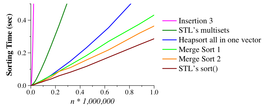
Dr. Plank also wrote merge_2_sort.cpp, which is identical to merge_1_sort, except that whenever size is less than 115, it sorts the array with insertion sort. The reason is that for small arrays, insertion sort is faster than merge sort, since it doesn't make recursive calls. Thus, merge_2_sort should be faster than merge_1_sort. (Dr. Plank determined the value of 115 experimentally). Dr. Plank compares these two implementations to four others below. Insertion 3 is a slightly more optimized version of Insertion 2 from last class. The STL multiset implementation is similar to what you likely used for Project01: multisets are stored internally as balanced binary trees. By performing n insertions, and then iterating through the multiset (aka in-order traversal of the binary tree), you effectively sort the numbers (just like Artists/Albums were output lexographically in your project). As you can see below its better than the optimized insertion sort but not as fast as the basic merge sort in Dr. Plank's experiments. I am not sure if these data were designed to work better with insertion sort, but even if they were merge sort usually wins/is faster on "typical" data as a O(n log n) algorithm (see above).
 |
Note the recursive call he uses, which is much like the call in merge sort at the beginning of these notes (no temp vector, though):
|
void recursive_sort(vector <double> &v, int start, int size, int print) |
In all versions of quicksort for a vector/arrays, Dr. Plank uses a slight variant of the "version with in-place partition," (from the Wikipedia notes). We'll start with Quicksort 1, where he simply uses the element in v[start] as the pivot. To perform the partition, he sets a left pointer at start+1 and a right pointer at start+size-1. While the left pointer is less than the right pointer, Dr. Plank does the following:
When we are done, he swaps the pivot in elements v[start] with the last element of the left set. Then he recursively sorts the left and right sets, omitting the pivot, since it is already in the correct place.
The output of quick_1_sort is similar to merge_1_sort: Dr. Plank prints the vector with an "S" label when he calls recursive_sort() with a size greater than 1. If the size is equal to two, he simply sorts the vector by hand and returns it. Otherwise, he partitions the vector around the pivot, then print the vector with a "P" label. This statement includes the index of the pivot element. At the end of sorting, he also prints out the vector.
Let's look at some example output:
UNIX> ./quick_1_sort 12
S:     0    12        5.77  5.26  6.49  0.43  6.09  4.95  3.15  3.46  7.55  6.82  6.69  3.62
P:     0    12     6  3.15  5.26  3.62  0.43  3.46  4.95  5.77  6.09  7.55  6.82  6.69  6.49
S:     0     6        3.15  5.26  3.62  0.43  3.46  4.95  5.77  6.09  7.55  6.82  6.69  6.49
P:     0     6     1  0.43  3.15  3.62  5.26  3.46  4.95  5.77  6.09  7.55  6.82  6.69  6.49
S:     0     1        0.43  3.15  3.62  5.26  3.46  4.95  5.77  6.09  7.55  6.82  6.69  6.49
S:     2     4        0.43  3.15  3.62  5.26  3.46  4.95  5.77  6.09  7.55  6.82  6.69  6.49
P:     2     4     3  0.43  3.15  3.46  3.62  5.26  4.95  5.77  6.09  7.55  6.82  6.69  6.49
S:     2     1        0.43  3.15  3.46  3.62  5.26  4.95  5.77  6.09  7.55  6.82  6.69  6.49
S:     4     2        0.43  3.15  3.46  3.62  5.26  4.95  5.77  6.09  7.55  6.82  6.69  6.49
S:     7     5        0.43  3.15  3.46  3.62  4.95  5.26  5.77  6.09  7.55  6.82  6.69  6.49
P:     7     5     7  0.43  3.15  3.46  3.62  4.95  5.26  5.77  6.09  7.55  6.82  6.69  6.49
S:     7     0        0.43  3.15  3.46  3.62  4.95  5.26  5.77  6.09  7.55  6.82  6.69  6.49
S:     8     4        0.43  3.15  3.46  3.62  4.95  5.26  5.77  6.09  7.55  6.82  6.69  6.49
P:     8     4    11  0.43  3.15  3.46  3.62  4.95  5.26  5.77  6.09  6.49  6.82  6.69  7.55
S:     8     3        0.43  3.15  3.46  3.62  4.95  5.26  5.77  6.09  6.49  6.82  6.69  7.55
P:     8     3     8  0.43  3.15  3.46  3.62  4.95  5.26  5.77  6.09  6.49  6.82  6.69  7.55
S:     8     0        0.43  3.15  3.46  3.62  4.95  5.26  5.77  6.09  6.49  6.82  6.69  7.55
S:     9     2        0.43  3.15  3.46  3.62  4.95  5.26  5.77  6.09  6.49  6.82  6.69  7.55
S:    12     0        0.43  3.15  3.46  3.62  4.95  5.26  5.77  6.09  6.49  6.69  6.82  7.55
                      0.43  3.15  3.46  3.62  4.95  5.26  5.77  6.09  6.49  6.69  6.82  7.55
UNIX>
|
Again, Dr. Plank has colored the part of the array under attention red/blue. When the size is greater than two and we are looking at an "S" line, the pivot is at v[start] and is colored blue. When you see a "P" line, the pivot will be at the given index, still colored blue, and recursive calls will be made to the left partition and the right partition. For example, in line one, the pivot is 5.77. The partition moves it to index 6, and then makes recursive calls with start=0,size=6 and start=7,size=5.
Lets consider two detailed examples of the partitioning algorithm. In the first, Dr Plank wants to show how the first partition above is done. To remind you, here is the array:
5.77 5.26 6.49 0.43 6.09 4.95 3.15 3.46 7.55 6.82 6.69 3.62 |
Our pivot is at element zero with a value of 5.77. What we do is have two integer indices, called left and right. Left starts at 1 and right starts at 11. We'll abbreviate left as L and right as R below, and he'll show two lines -- the original vector, and what is looks like as it is being partitioned:
Original:     5.77  5.26  6.49  0.43  6.09  4.95  3.15  3.46  7.55  6.82  6.69  3.62
In Progress:  5.77  5.26  6.49  0.43  6.09  4.95  3.15  3.46  7.55  6.82  6.69  3.62
              Pivot L=1                                                         R=11
|
Now, our first step is to increment L until it is pointing to a value ≥ the pivot. We'll color the skipped-over value green:
Original:     5.77  5.26  6.49  0.43  6.09  4.95  3.15  3.46  7.55  6.82  6.69  3.62
In Progress:  5.77  5.26  6.49  0.43  6.09  4.95  3.15  3.46  7.55  6.82  6.69  3.62
              Pivot       L=2                                                   R=11
|
Next, lets decrement R until it is pointing to a value ≤ the pivot. Since it is already pointing to such a value, we do not need to decrement it at all. Note, this picture is the same as the previous one:
Original:     5.77  5.26  6.49  0.43  6.09  4.95  3.15  3.46  7.55  6.82  6.69  3.62
In Progress:  5.77  5.26  6.49  0.43  6.09  4.95  3.15  3.46  7.55  6.82  6.69  3.62
              Pivot       L=2                                                   R=11
|
We swap the values pointed to by L and R, increment L and decrement R. The elements in the right partition will now be colored purple.
Original:     5.77  5.26  6.49  0.43  6.09  4.95  3.15  3.46  7.55  6.82  6.69  3.62
In Progress:  5.77  5.26  3.62  0.43  6.09  4.95  3.15  3.46  7.55  6.82  6.69  6.49
              Pivot             L=3                                       R=10
|
And we repeat. Increment L until it is pointing to a value ≥ the pivot:
Original:     5.77  5.26  6.49  0.43  6.09  4.95  3.15  3.46  7.55  6.82  6.69  3.62
In Progress:  5.77  5.26  3.62  0.43  6.09  4.95  3.15  3.46  7.55  6.82  6.69  6.49
              Pivot                   L=4                                 R=10
|
Decrement R until it is pointing to a value ≤ the pivot:
Original:     5.77  5.26  6.49  0.43  6.09  4.95  3.15  3.46  7.55  6.82  6.69  3.62
In Progress:  5.77  5.26  3.62  0.43  6.09  4.95  3.15  3.46  7.55  6.82  6.69  6.49
              Pivot                   L=4               R=7
|
Swap, increment L and decrement R:.
Original:     5.77  5.26  6.49  0.43  6.09  4.95  3.15  3.46  7.55  6.82  6.69  3.62
In Progress:  5.77  5.26  3.62  0.43  3.46  4.95  3.15  6.09  7.55  6.82  6.69  6.49
              Pivot                         L=5   R=6
|
Repeat again. Increment L until it is pointing to a value ≥ the pivot:
Original:     5.77  5.26  6.49  0.43  6.09  4.95  3.15  3.46  7.55  6.82  6.69  3.62
In Progress:  5.77  5.26  3.62  0.43  3.46  4.95  3.15  6.09  7.55  6.82  6.69  6.49
              Pivot                               R=6   L=7
|
Decrement R until it is pointing to a value ≤ the pivot (it is already doing that, so this picture is identical to the last): :
Original:     5.77  5.26  6.49  0.43  6.09  4.95  3.15  3.46  7.55  6.82  6.69  3.62
In Progress:  5.77  5.26  3.62  0.43  3.46  4.95  3.15  6.09  7.55  6.82  6.69  6.49
              Pivot                               R=6   L=7
|
Because L is greater than R, we're done. We now swap the pivot with the last element in the left (green) set:
Original:     5.77  5.26  6.49  0.43  6.09  4.95  3.15  3.46  7.55  6.82  6.69  3.62
In Progress:  3.15  5.26  3.62  0.43  3.46  4.95  5.77  6.09  7.55  6.82  6.69  6.49
                                                  R=6   L=7
|
And we make two recursive calls:
recursive_sort(v, 0, 6, print);
recursive_sort(v, 7, 5, print);
As you can see, this matches the first "P" line in the input above. Additionally, you can see the two recursive calls at lines 3 and 10.
PAY ATTENTION TO THIS: There are times when, after incrementing and decrementing, you will have L equal to R. Pay attention to this case, and perform the appropriate action. We'll assess this in your solutions with at least one test case.
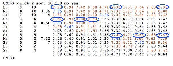 |
The circles show the three elements considered for the pivot -- the one with the median value is always chosen. (The indices are calculated as start, (start+size-1) and (start+size/2).
This makes a minor difference in sorting random lists, but a huge difference in sorting presorted lists:
UNIX> time ./quick_1_sorted 100000 1 0 no no
5.173u 0.012s 0:05.21 99.4%     0+0k 0+0io 0pf+0w
UNIX> time ./quick_2_sorted 100000 1 0 no no
0.006u 0.003s 0:00.01 0.0%      0+0k 0+0io 0pf+0w
UNIX>
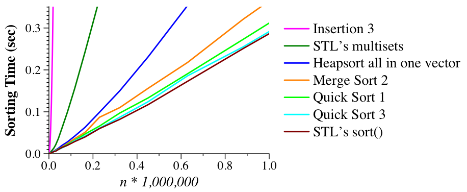
Quicksort #3 sorts lists of size 46 and smaller with insertion sort. That improves the performance a little. Heapsort is something we'll talk about next week; as we'll discuss, its better than multiset/balanced tree but not as good as merge sort (and the experiments support that assertion -- see below)
 |
If our input has a known probability distribution (e.g., randomly uniformly and at random over some interval), or has a limited number of values (e.g., small integers) we can use a sort known as bucket sort.
The small integer version is simple and we'll discuss it in class.
As for for random numbers, as a concrete example, consider 1000 random numbers generated between 0 and 10.
Now suppose we see the value 4.53. Since we know the probability distribution of drand48()*10 is uniform between 0 and ten, we know that the value 4.53 is going to be pretty near element 453 when the vector is sorted.
A first pass of using this information is in bucket_1_sort.cpp
/* Headers and insertion sort omitted. */
void sort_doubles(vector <double> &v, int print)
{
  int sz;
  int index, j;
  double val;
  double *v2;
  int hind, lind, done, i;

  sz = v.size();

  /* Allocate a new array, and set every entry to -1. */

  v2 = (double *) malloc(sizeof(double)*sz);
  for (i = 0; i < sz; i++) v2[i] = -1;

  /* For each element, find out where you think it will go.
     If that index is empty, put it there. */

  for (i = 0; i < sz; i++) {
    val = (v[i] * sz/10.0);
    index = (int) val;
    if (v2[index] == -1) {
      v2[index] = v[i];

    /* Otherwise, check nearby, above and below, until
       you find an empty element. */
|
    } else {
      hind = index+1;
      lind = index-1;
      done = 0;
      while(!done) {
        if (hind < sz && v2[hind] == -1) {
          v2[hind] = v[i];
          done = 1;
        } else {
          hind++;
        }
        if (!done && lind >= 0 && v2[lind] == -1) {
          v2[lind] = v[i];
          done = 1;
        } else {
          lind--;
        }
      }
    }
  }

  /* At the end, copy this new vector back to the
     old one, free it, and call insertion sort to
     "clean up" the vector. */

  for (i = 0; i < sz; i++) v[i] = v2[i];
  free(v2);

  if (print) {
    cout << "Before Insertion Sort\n";
    for (j = 0; j < v.size(); j++) printf("%.2lf ", v[j]);
    cout << endl;
  }

  insertion_sort(v);

  if (print) {
    cout << "After Insertion Sort\n";
    for (j = 0; j < v.size(); j++) printf("%.2lf ", v[j]);
    cout << endl;
  }
}
|
What this code does is predict where each value is going to go, and then put it into that index of v2 so long as it's empty (-1). If that entry is not empty, then it looks adjacent to that entry, and continues doing so until it finds an empty slot, and puts it there. Once that process is done, it copies v2 back to v and uses insertion sort to sort v.
Since v is nearly sorted (or should be), insertion sort should sort it very quickly.
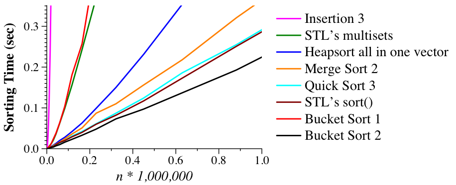
As it turns out, howerver, this process is quite slow because as v2 fills up, it takes longer to find empty slots, and as a result they are quite far from where they should be. Similar to what you may have done with hash tables, we will "fix" this in bucket_2_sort.cpp where we double the size of v2 so that there are more empty cells and a much smaller chance of having to move to adjacent cells (aka a collision).
As you can see, the results are great -- even better than the Standard Template Library!
 |