 |
The Disjoint Set data structure solves a specific problem that is interesting both theoretically and practically. The problem is as follows:
You have a collection of n items, which you number from 0 to n-1. These items will be partitioned into some number of sets. The sets are "disjoint" which means that no item belongs to more than one set. All items belong to some set though (hence the use of the word "partition.").
There are two operations that you can perform:
Disjoint sets are very useful in connected component applications. They are also extremely efficient, which will be discussed later.
When a node has a NULL link, we call it the "root" of a set. If you call Find() on a node with a NULL link, it will return the node's item number, and that is the set id of the node. Therefore, when you first start, every node is the root of its own set, and when you call Find(i), it will return i.
When you call Union(i, j), remember that i and j must be set id's. Therefore, they must be nodes with NULL links. What you do is have one of those nodes set its link to the other node.
Let's illustrate with a simple example. We initialize an instance of disjoint sets with 10 items. Each item is a node with a number from 0 to 9. Each node has a NULL link, which we depict by not drawing any arrows from the node:
 |
Again, each node is in its own set, and each node's set id is its number. Suppose we call Union(0, 1), Union(2, 3) and Union(4, 5). These will each set one of the node's link to the other node. We'll talk about how that gets done later. However, suppose this is the result:
 |
As you can see, node 0's link has been set to 1. Both of these nodes' set ids are now 1, which means Find(0) equals Find(1) equals one. Similarly, Find(2) equals Find(3) equals three.
This gives you a clue about implementing Find(). When you call Find(n), what you do is keep setting n to n's link, until n's link is NULL. At that point, you are at the root of the set, and you return n.
Union is pretty simple, too, but you have some choices about how to determine which node sets its link field to the other. We use three methods to do this:
As always, a picture helps. Suppose this is the state of our disjoint set instance:
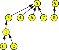 |
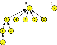
There are two sets, with set id's 5 and 9. Now, suppose you call Find(0). It will return five, but along the way to the root node of its set, it encounters nodes 1 and 3. Before returning five, it sets the links to 0, 1 and 3 to five:
 |
Do you see why this is a good thing? Previously, when you called Find(0), you needed to travel through nodes 1 and 3 before getting to 5. If you call Find(0) again, you get to node 5 directly. Similarly, you have improved the performance of Find(1), and Find(2).
You can see that path compression has altered the height of the set. However, we maintain what its height would be, had we not used path compression, and call it the set's rank. We use the rank to determine how we perform union.
#pragma once
#include <vector>
using namespace std;

/* The Disjoint Set API is defined as a c++
   interface, because I am implementing it three
   ways.  Each subclass implementation is in its
   own cpp file.  */

class DisjointSet {
  public:
    virtual ~DisjointSet() {};
    virtual int Union(int s1, int s2) = 0;
    virtual int Find(int element) = 0;
    virtual void Print() = 0;
};

/* The first subclass implements Union-by-Size. */

class DisjointSetBySize : public DisjointSet {
  public:
    DisjointSetBySize(int nelements);
    int Union(int s1, int s2);
    int Find(int element);
    void Print();

  protected:
    vector <int> links;
    vector <int> sizes;
};
| /* The second subclass implements Union-by-Height. */
class DisjointSetByHeight : public DisjointSet {
public:
DisjointSetByHeight(int nelements);
int Union(int s1, int s2);
int Find(int element);
void Print();
protected:
vector <int> links;
vector <int> heights;
};
/* The third subclass implements Union-by-Rank
with path compression. */
class DisjointSetByRankWPC : public DisjointSet {
public:
DisjointSetByRankWPC(int nelements);
int Union(int s1, int s2);
int Find(int element);
void Print();
protected:
vector <int> links;
vector <int> ranks;
};
|
Each subclass has a links vector that holds the parent pointers for each element. If links[e] is equal to negative one, then e is the root and set id of the set. If links[e] does not equal -1, then the set id of e is equal to the set id of links[e].
Each subclass, however, has a different vector to store the sizes/heights/ranks:
In all cases, if e is not the root of a set, sizes[e]/heights[e]/ranks[e] is immaterial.
Each subclass is implemented in its own source file:
The constructor sets up the two vectors. Each element is in its own set, so all links are -1 and all sizes are 1.
DisjointSetBySize::DisjointSetBySize(int nelements)
{
  links.resize(nelements, -1);
  sizes.resize(nelements, 1);
}
|
The Find(e) operator chases link[e] until it equals -1:
int Disjoint::Find(int element)
{
  while (links[element] != -1) element = links[element];
  return element;
}
|
And the Union(s1, s2) operator first checks to make sure that the set id's are valid, and then chooses a parent and a child from s1 and s2. The parent will be the one with the bigger of the two sets. It changes the link field of the child to point to the parent, and then it updates the size of the parent in the sizes vector:
int Disjoint::Union(int s1, int s2)
{
  int p, c;

  if (links[s1] != -1 || links[s2] != -1) {
    cerr << "Must call union on a set, and not just an element.\n";
    exit(1);
  }
  if (sizes[s1] > sizes[s2]) {
    p = s1;
    c = s2;
  } else {
    p = s2;
    c = s1;
  }
  links[c] = p;
  sizes[p] += sizes[c];    /* HERE */
  return p;
}
|
I won't show Print(): it simply prints out the vectors.
The only difference between union-by-size and union-by-height is that heights keeps track of the number of nodes in the longest path. After changing all of the "sizes" to "heights", it is a one line change to union-by-size -- the line marked HERE is changed to:
if (heights[s1] == heights[s2]) heights[p]++; |
This is because a set's height only changes if the two sets being merged have equal heights.
Finally, union-by-rank is equivalent to union-by-height, except that you perform path compression on find operations. With path compression, each time you perform a Find(e) operation, you update the links field of all elements on the path to the root, so that they equal the root. Here's one way to do this:
int Disjoint::Find(int element)
{
  vector <int> q;
  int i;

  while (links[element] != -1) {
    q.push_back(element);
    element = links[element];
  }
  for (i = 0; i < q.size(); i++) links[q[i]] = element;
  return element;
}
|
This is one of those convenient things about the STL -- I don't have to call new or delete. When the Find() operation is over, the vector is deallocated.
However, I could implement path compression in two other ways, and it's illustrative to go over them. The first is with simple recursion:
int Disjoint::Find(int element)
{
  if (links[element] == -1) return element;
  links[element] = Find(links[element]);
  return links[element];
}
|
The second is to traverse links to the root, but while doing so, setting links[element] to be element's child. In that way, once you find the root, you can use links to go back to the original element, performing path compression along the way. The code is here -- if you're a little leery of this code, copy it to your directory and put in some print statements. This should be the best implementation performance-wise, because it doesn't use extra memory like the other two.
int Disjoint::Find(int e)
{
  int p, c;   // P is the parent, c is the child.
  c = -1;

  /* Find the root of the tree, but along the way, set
     the parents' links to the children. */

  c = -1;
  while (links[e] != -1) {
    p = links[e];
    links[e] = c;
    c = e;
    e = p;
  }

  /* Now, travel back to the original element, setting
     every link to the root of the tree. */

  p = e;
  e = c;
  while (e != -1) {
    c = links[e];
    links[e] = p;
    e =c;
  }
  return p;
}
|
int main(int argc, char **argv)
{
  DisjointSet *d;
  string arg;

  int s01, s23, s45;
  int s0123, s456, s4567, s45678;
  int s012345678;

  /* Error check the command line. */
  arg = "";
  if (argc == 2) arg = argv[1];

  if (arg != "size" && arg != "height" && arg != "rank") {
    fprintf(stderr, "usage: example size|height|rank\n");
    exit(1);
  }

  /* Create the DisjointSet pointer using the proper subclass constructor. */
  switch(arg[0]) {
    case 's': d = new DisjointSetBySize(10); break;
    case 'h': d = new DisjointSetByHeight(10); break;
    case 'r': d = new DisjointSetByRankWPC(10); break;
    default: exit(1);
  }
|
As for the rest, I'm just going to show the Union and Find commands, so that see what it's doing without all of the prints:
s01 = d->Union(0, 1); s23 = d->Union(2, 3); s45 = d->Union(4, 5); d->Print(); print d->Find(0) and d->Find(1)); s0123 = d->Union(s01, s23); s456 = d->Union(s45, 6); s4567 = d->Union(s456, 7); s45678 = d->Union(s4567, 8); print d->Find(1); print d->Find(2); print d->Find(4); print d->Find(7); d->Print(); s012345678 = d->Union(s0123, s45678); d->Print(); print d->Find(3); print d->Find(5); print d->Find(7); d->Print(); print d->Find(0); d->Print(); } |
The makefile compiles eveything:
UNIX> make clean
rm -f *.o a.out example
UNIX> make example
g++ -c -O example.cpp
g++ -c -O disjoint-height.cpp
g++ -c -O disjoint-rank.cpp
g++ -c -O disjoint-size.cpp
g++ -O -o example example.o disjoint-height.o disjoint-rank.o disjoint-size.o
UNIX>
We first run it with union-by-size. Let's look at the output incrementally. When the program starts, it sets up an empty Disjoint with ten elements:
UNIX> ./example size Starting State: Node: 0 1 2 3 4 5 6 7 8 9 Links: -1 -1 -1 -1 -1 -1 -1 -1 -1 -1 Sizes: 1 1 1 1 1 1 1 1 1 1 |
 |
Next, it performs three union operations: Union(0, 1), Union(2, 3), and Union(4, 5). Since each set in all three operations is the same size, the choice of parent and child is arbitrary. Here's the output and how it looks pictorally (I've added the sizes to the roots of each set):
Doing d->Union(0, 1). Resulting set = 1 Doing d->Union(2, 3). Resulting set = 3 Doing d->Union(4, 5). Resulting set = 5 Node: 0 1 2 3 4 5 6 7 8 9 Links: 1 -1 3 -1 5 -1 -1 -1 -1 -1 Sizes: 1 2 1 2 1 2 1 1 1 1 |
 |
Next it performs four more union operations: Union(1, 3), Union(5, 6), Union(5, 7), and Union(5, 8). The first union operation merges two sets of the same size, so the parent/child selection is arbitrary. The remaining three union operations merge sets of size 1 (sets 6, 7 and 8) with set 5 which is larger. Thus, in each case, set 5 becomes the parent. The resulting sets are pictured to the right.
The Find() operations return the root of each set -- three in the set {0, 1, 2, 3}, and five in the set {4, 5, 6, 7, 8}.
You should make sure that you understand how the output of the program maps to the picture. In particular, make sure you understand the Links and Ranks lines and what they mean.
Doing d->Union(1, 3). Resulting set = 3 Doing d->Union(5, 6). Resulting set = 5 Doing d->Union(5, 7). Resulting set = 5 Doing d->Union(5, 8). Resulting set = 5 d->Find(1) = 3 d->Find(2) = 3 d->Find(4) = 5 d->Find(7) = 5 Node: 0 1 2 3 4 5 6 7 8 9 Links: 1 3 3 -1 5 -1 5 5 5 -1 Sizes: 1 2 1 4 1 5 1 1 1 1 |
 |
Now, we perform Union(3, 5). Since set 5 has more elements than set 3, it is the parent and 3 is the child. Subsequent Find() operations on 3, 5, 7 and 0 all return 5 as the set id:
Doing d->Union(3, 5). Resulting set = 5 Node: 0 1 2 3 4 5 6 7 8 9 Links: 1 3 3 5 5 -1 5 5 5 -1 Sizes: 1 2 1 4 1 9 1 1 1 1 d->Find(3) = 5 d->Find(5) = 5 d->Find(7) = 5 Node: 0 1 2 3 4 5 6 7 8 9 Links: 1 3 3 5 5 -1 5 5 5 -1 Sizes: 1 2 1 4 1 9 1 1 1 1 d->Find(0) = 5 Node: 0 1 2 3 4 5 6 7 8 9 Links: 1 3 3 5 5 -1 5 5 5 -1 Sizes: 1 2 1 4 1 9 1 1 1 1 UNIX> |
 |
UNIX> ./example height Starting State: Node: 0 1 2 3 4 5 6 7 8 9 Links: -1 -1 -1 -1 -1 -1 -1 -1 -1 -1 Hghts: 1 1 1 1 1 1 1 1 1 1 |
 |
Doing d->Union(0, 1). Resulting set = 1 Doing d->Union(2, 3). Resulting set = 3 Doing d->Union(4, 5). Resulting set = 5 Node: 0 1 2 3 4 5 6 7 8 9 Links: 1 -1 3 -1 5 -1 -1 -1 -1 -1 Hghts: 1 2 1 2 1 2 1 1 1 1 |
 |
Doing d->Union(1, 3). Resulting set = 3 Doing d->Union(5, 6). Resulting set = 5 Doing d->Union(5, 7). Resulting set = 5 Doing d->Union(5, 8). Resulting set = 5 d->Find(1) = 3 d->Find(2) = 3 d->Find(4) = 5 d->Find(7) = 5 Node: 0 1 2 3 4 5 6 7 8 9 Links: 1 3 3 -1 5 -1 5 5 5 -1 Hghts: 1 2 1 3 1 2 1 1 1 1 |
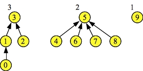 |
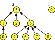
Although the trees look the same, the heights fields are different from the previous size fields. So, when we perform the last union of 3 and 5, 3 becomes the parent, since it has greater height. Subsequent Find() operations all return 3 now:
Doing d->Union(3, 5). Resulting set = 3 Node: 0 1 2 3 4 5 6 7 8 9 Links: 1 3 3 -1 5 3 5 5 5 -1 Hghts: 1 2 1 3 1 2 1 1 1 1 d->Find(3) = 3 d->Find(5) = 3 d->Find(7) = 3 Node: 0 1 2 3 4 5 6 7 8 9 Links: 1 3 3 -1 5 3 5 5 5 -1 Hghts: 1 2 1 3 1 2 1 1 1 1 d->Find(0) = 3 Node: 0 1 2 3 4 5 6 7 8 9 Links: 1 3 3 -1 5 3 5 5 5 -1 Hghts: 1 2 1 3 1 2 1 1 1 1 UNIX> |
 |
UNIX> ./example rank .... .... Doing d->Union(3, 5). Resulting set = 3 Node: 0 1 2 3 4 5 6 7 8 9 Links: 1 3 3 -1 5 3 5 5 5 -1 Ranks: 1 2 1 3 1 2 1 1 1 1 |
 |
When we perform the three Find() operations, the last one -- Find(7) performs path compression, setting node 7's link to the root of the set: 3:
d->Find(3) = 3 d->Find(5) = 3 d->Find(7) = 3 Node: 0 1 2 3 4 5 6 7 8 9 Links: 1 3 3 -1 5 3 5 3 5 -1 Ranks: 1 2 1 3 1 2 1 1 1 1 |
 |
Similarly, the last Find(0) operation also performs path compression:
d->Find(0) = 3 Node: 0 1 2 3 4 5 6 7 8 9 Links: 3 3 3 -1 5 3 5 3 5 -1 Ranks: 1 2 1 3 1 2 1 1 1 1 |
 |
Were we to call Find(4) Find(6) and Find(8), then those nodes too would perform path compression and point directly to node three. In that case, the state would be the following:
d.Find(4) = 3 d.Find(6) = 3 d.Find(8) = 3 Node: 0 1 2 3 4 5 6 7 8 9 Links: 3 3 3 -1 3 3 3 3 3 -1 Ranks: 1 2 1 3 1 2 1 1 1 1 |
 |
I draw this picture because you should see that ranks[3] remains at three, even though its height is two. This is because the ranks field traces what the height of the tree would be with no path compression. We can't keep it updated properly without adding to the running time of the Union() or Find() operations. Fortunately, it doesn't matter -- the fine theoreticians of the world have proved that Find() operations run in O(α(n)) time. Union() operations are still O(1).
 |
A good maze is one where the graph is fully connected, so that every cell is reachable from the start/end cells, but there are no cycles. We can generate such a maze using disjoint sets. We start with a completely disconnected graph, where each cell is surrounded by walls. If this graph has r rows and c columns, then the graph contains r*c nodes and no edges.
What we'll do is choose a random wall to remove. If that wall separates nodes in different connected components, then we'll remove it, thereby lowering the number of connected components. If it doesn't separate nodes in different connected components, we keep it.
This can be done with disjoint sets. We start with each cell in its own set, and then we choose a random wall. If that wall connects two nodes in different sets, we remove the wall and call Union() on the two sets. Otherwise, we keep the wall. We keep doing this until we have just one set.
The code is in maze-gen.cpp. It's a little tricky. We first generate all the walls. Walls that separate vertically adjacent cells are indexed by the smaller cell number. Walls that separate horizontally adjacent cells are indexed by the smaller cell number plus r*c. We generate all the walls and insert them into a multiset keyed by a random number. Then we traverse the multiset, deleting walls if they separate different components, until we have just one component. Then we print out the walls:
#include <vector>
#include <cstdlib>
#include <cstdio>
#include <map>
#include "disjoint.h"
#include <iostream>
using namespace std;

int main(int argc, char **argv)
{
  int r, c, row, column, c1, c2, ncomp, s1, s2, hov;
  DisjointSet *d;
  map <double, int> walls;
  map <double, int>::iterator wit;
  map <double, int>::iterator tmp;

  /* Parse the command line and create the instance of the disjoint set. */

  if (argc != 4) {
    fprintf(stderr, "usage mazegen rows cols size|height|rank\n"); exit(1); }

  r = atoi(argv[1]);
  c = atoi(argv[2]);

  switch(argv[3][0]) {
    case 's': d = new DisjointSetBySize(r*c); break;
    case 'h': d = new DisjointSetByHeight(r*c); break;
    case 'r': d = new DisjointSetByRankWPC(r*c); break;
    default: fprintf(stderr, "Bad last argument.  Should be s|h|r.\n"); exit(1);
  }

  /* Generate walls that separate vertical cells. */

  for (row = 0; row < r-1; row++) {
    for (column = 0; column < c; column++) {
      c1 = row*c + column;
      walls.insert(make_pair(drand48(), c1));
    }
  }

  /* Generate walls that separate horizontal cells. */

  for (row = 0; row < r; row++) {
    for (column = 0; column < c-1; column++) {
      c1 = (row*c + column) + r*c;
      walls.insert(make_pair(drand48(), c1));
    }
  }

  /* Run through the walls map, deleting walls when they
     separate cells in different disjoint sets. */

  ncomp = r*c;
  wit = walls.begin();
  while (ncomp > 1) {
    c1 = wit->second;
    if (c1 < r*c) {    // This is a wall separating vertical cells.
      c2 = c1 + c;
    } else {           // This is a wall separating horizontal cells.
      c1 -= r*c;
      c2 = c1+1;
    }
    s1 = d->Find(c1);
    s2 = d->Find(c2);
    if (s1 != s2) {     // Test for different connected components.
      d->Union(s1, s2);
      tmp = wit;
      wit++;
      walls.erase(tmp);
      ncomp--;
    } else {
      wit++;
    }
  }

  /* Print out the remaining walls. */

  printf("ROWS %d COLS %d\n", r, c);

  for (wit = walls.begin(); wit != walls.end(); wit++) {
    c1 = wit->second;
    if (c1 < r*c) {
      c2 = c1 + c;
    } else {
      c1 -= r*c;
      c2 = c1+1;
    }
    printf("WALL %d %d\n", c1, c2);
  }
  return 0;
}
|
We can run this and pipe the output to the program maze_ppm (from a CS302 lab that you may not have done yet), and that lets us generate mazes of all sizes:
UNIX> ./maze-gen 50 100 rank | maze_ppm 5 | convert - maze2.jpg 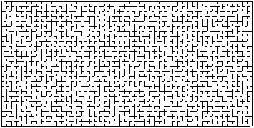 |
#include <vector>
#include <cstdlib>
#include <cstdio>
#include "disjoint.h"
#include <iostream>
using namespace std;

int main()
{
  DisjointSet *d;
  int s01, s23, s45, s67;

  d = new DisjointSetByRankWPC(8);

  s01 = d->Union(0, 1);
  s23 = d->Union(2, 3);
  s45 = d->Union(4, 5);
  s67 = d->Union(6, 7);

  s01 = d->Union(s01, s23);
  s45 = d->Union(s45, s67);

  s01 = d->Union(s01, s45);

  d->Print();

  printf("\n");

  d->Find(0);

  d->Print();
  exit(0);
}
|
When I compile this with DJ-rank.cpp and run it, the first lines are:
UNIX> example-exam

Elts:   0  1  2  3  4  5  6  7
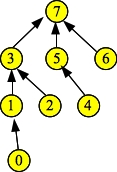
Links:  1  3  3  7  5  7  7 -1
Ranks:  1  2  1  3  1  2  1  4
Draw the data structure (as circles and pointers) just before the d.Find() call. Then give me the output of the last d.Print() call.
 |
When you call d.Find(0), path compression occurs, which means that nodes 0, 1 (and 3) all point to the root (7):
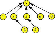 |
Thus, the links fields for 0 and 1 will become 7. Everything else remains the same, because Find() doesn't change the ranks. So the output is:
Elts:   0  1  2  3  4  5  6  7
Links:  7  7  3  7  5  7  7 -1
Ranks:  1  2  1  3  1  2  1  4