G1: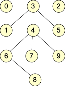 |
G2: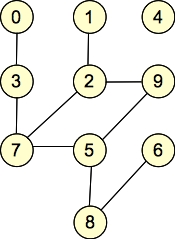 |
Wikipedia has a glossary of graph terms. The terms you should know are the following: vertices, edges, adjacency, incidence, directed/undirected, path, cycle, loop, multiedge, connected component, bipartite.
Let's give some examples. Here are two graphs, which we will call G1 and G2:
G1: |
G2: |
They are undirected graphs. G1 has four connected components and no cycles, while G2 has two connected components and one cycle. Both graphs are bipartite: with G1, the two sets of nodes are { 0, 1, 2, 5, 6, 7, 9 }, { 3, 4, 8 }. Other partitionings are possible (for example, nodes 0 and 2 can go into either set). For G2, the two sets are { 0, 1, 4, 7, 8, 9 }, { 2, 3, 5, 6 }. (You can put 4 into either set, but beyond that, the two sets are fixed).
Were we to add the edge (0, 1) to G2, it would no longer be bipartite.
If our adjacency lists contain indices of nodes, then the following table shows the adjacency list representation of the graph:
| Node | Adjacency list in G1 | Adjacency list in G2 |
| 0 | {} | { 3 } |
| 1 | { 3 } | { 2 } |
| 2 | {} | { 1, 9, 7 } |
| 3 | { 1, 5 } | { 0, 7 } |
| 4 | { 6, 7, 9 } | {} |
| 5 | { 3 } | { 9, 7, 8 } |
| 6 | { 4, 8 } | { 8 } |
| 7 | { 4 } | { 2, 3, 5 } |
| 8 | { 6 } | { 5, 6 } |
| 9 | { 4 } | { 2, 5 } |
With undirected graphs, we typically store each edge twice.
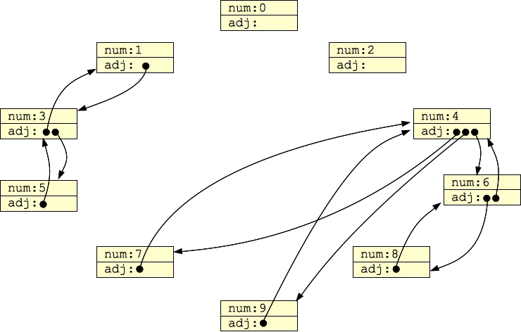
On the other hand, you could have each node be its own data structure, and have each adjacency list be (for example a vector of) pointers to nodes like this:
struct Node {
    int num;
    vector <Node *> adj;
};
|
Then, G1 above would look as follows when it is stored in computer memory:
 |
Here are the adjacency matrices for the two example graphs:
Adjacency Matrix for G1
     0  1  2  3  4  5  6  7  8  9
    -- -- -- -- -- -- -- -- -- --
 0 | 0  0  0  0  0  0  0  0  0  0
 1 | 0  0  0  1  0  0  0  0  0  0
 2 | 0  0  0  0  0  0  0  0  0  0
 3 | 0  1  0  0  0  1  0  0  0  0
 4 | 0  0  0  0  0  0  1  1  0  1
 5 | 0  0  0  1  0  0  0  0  0  0
 6 | 0  0  0  0  1  0  0  0  1  0
 7 | 0  0  0  0  1  0  0  0  0  0
 8 | 0  0  0  0  0  0  1  0  0  0
 9 | 0  0  0  0  1  0  0  0  0  0
|
Adjacency Matrix for G2
     0  1  2  3  4  5  6  7  8  9
    -- -- -- -- -- -- -- -- -- --
 0 | 0  0  0  1  0  0  0  0  0  0
 1 | 0  0  1  0  0  0  0  0  0  0
 2 | 0  1  0  0  0  0  0  1  0  1
 3 | 0  0  0  1  0  0  0  1  0  0
 4 | 0  0  0  0  0  0  0  0  0  0
 5 | 0  0  0  0  0  0  0  1  1  1
 6 | 0  0  0  0  0  0  0  0  1  0
 7 | 0  0  1  1  0  1  0  0  0  0
 8 | 0  0  0  0  0  1  1  0  0  0
 9 | 0  0  1  0  0  1  0  0  0  0
|
Because this is an undirected graph, each edge has two entries in the adjacency matrix. It also means that the adjacency matrices are symmetric around the diagonal of the matrix.
If we let |V| be the number of nodes, and |E| be the number of edges (we'll see why we use those terms later), then adjacency lists consume O(|E|) of memory, while adjacency matrices consume O(|V|2) of memory. For that reason, we typically use adjacency matrices either when the graphs are so small that the size of the matrix doesn't matter, or when the graph is very dense, which means that |E| is O(|V|2), and the matrix and list representations use roughly the same amount of memory.
V is a collection of vertices, and E is a collection of edges. E is not a mathematically definable set, but its easier to think of both V and E as sets for now.
Because they are both effectively sets in these notes, you denote the size of V, and therefore the number of vertices as |V|. Similarly, the number of edges is |E|.
The specification of V and E defines the graph. For example, here is a mathematical definition of G1:
The mathematical representation can be very powerful, albeit a little terse and sometimes hard to read. For example, recall the binary heap implementation of priority queues from last week. Those data can be viewed as a graph where it's clear where the nodes and edges are. You'll review this on the current challenged.
Here's an example from Dr. Plank's lecture notes:
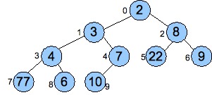 |
This lends itself to a beautiful mathematical definition:
g1.txt
NNODES 10 EDGE 4 9 EDGE 4 6 EDGE 4 7 EDGE 6 8 EDGE 3 5 EDGE 1 3 |
g2.txt
NNODES 10 EDGE 5 9 EDGE 1 2 EDGE 5 8 EDGE 3 7 EDGE 2 7 EDGE 0 3 EDGE 5 7 EDGE 6 8 EDGE 2 9 |
We can specify the edges in any order; what matters is each desired edge has an entry in this file.