Golub-Kahan-Lanczos Bidiagonalization Procedure.

Next: Relationship to Symmetric Lanczos. Up: Golub-Kahan-Lanczos Method Previous: Golub-Kahan-Lanczos Method Contents Index

Golub-Kahan-Lanczos Bidiagonalization Procedure.

As discussed in §6.2, the first phase of a transformation method for the SVD is to compute unitary matrices

and

such that

is in bidiagonal form. In fact, the first column

can be chosen as an arbitrary unit vector, after which the other columns of

and

are generally determined uniquely. We write this as

$\begin{displaymath} U^{*} A V = B = \left[ \begin{array}{cccccc} \alpha_1 & \be... ...\beta_{n-1} \\ & & & & &\alpha_{n} \\ \end{array} \right]. \end{displaymath}$

(111)

All $\alpha$ s and $\beta$ s are real even if

was complex.

The constants $\alpha_k$ and $\beta_k$ are given by

$\begin{displaymath} \alpha_k = u^{\ast}_k A v_k \quad\mbox{and}\quad \beta_k = u^{\ast}_k A v_{k+1}. \end{displaymath}$

From the bidiagonal form (6.4) we may derive a double recursion for the columns

and

. Multiplying by

, we have

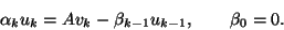
$\begin{displaymath} A \left[\begin{array}{cccc} v_1 & v_2 & \ldots & v_n \e... ... & \beta_{n-1} \\ & & & & \alpha_n \\ \end{array} \right]. \end{displaymath}$

Equating the

th columns on both sides, we get

$\begin{displaymath} Av_k = \beta_{k-1}u_{k-1} + \alpha_k u_k \end{displaymath}$

$\begin{displaymath} \alpha_k u_k = Av_k - \beta_{k-1}u_{k-1}, \quad\quad \beta_0 = 0. \end{displaymath}$

(112)

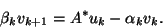
On the other hand, from the relation

$\begin{displaymath} A^{\ast} \left[\begin{array}{cccc} u_1 & u_2 & \ldots & u_n... ... & \\ & & & \beta_{n-1} & \alpha_n \\ \end{array} \right], \end{displaymath}$

we get

$\begin{displaymath} A^{\ast} u_k = {\alpha}_k v_k + {\beta}_k v_{k+1} \end{displaymath}$

$\begin{displaymath} {\beta}_k v_{k+1} = A^{\ast} u_k - {\alpha}_k v_k. \end{displaymath}$

(113)

Since the columns of and are normalized, we must have

$\begin{displaymath} \alpha_k = \Vert Av_k - \beta_{k-1}u_{k-1}\Vert _2 \end{displaymath}$

and

$\begin{displaymath} \beta_k = \Vert A^* u_k - \alpha_k v_k\Vert _2. \end{displaymath}$

We summarize the recursion in the following algorithm.

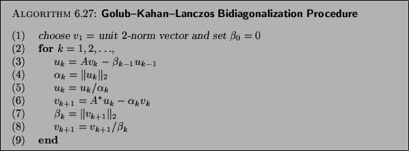
$\begin{algorithm}{Golub--Kahan--Lanczos Bidiagonalization Procedure } { \begin{t... ...} = v_{k+1}/ \beta_k$\ \\ {\rm (9)}\> {\bf end} \end{tabbing}} \end{algorithm}$

Collecting the computed quantities from the first steps of the algorithm, we have the following important relations:

$\displaystyle A V_k$	$\textstyle =$	$\displaystyle U_k B_k,$	(114)
$\displaystyle A^{\ast} U_{k}$	$\textstyle =$	$\displaystyle V_k B^_k + \beta_{k}v_{k+1}e^_k,$	(115)