ESTIMATING DEPENDENCIES FROM SPATIAL AVERAGES

The value of such functions can be predicted by first estimating the dependence structure of the underlying stochastic process. Our proposed method for estimating the covariance function from the integrals of a stationary isotropic stochastic process poses the problem as a set of integral equations. To test this proposal we applied it to epidemiological data on the incidence rates of three diseases in the United States between 1980 and 1994. Spatial correlations obtained in this way reasonably described the mechanism by which those diseases spread. We therefore conclude that it is possible to reliably estimate covariance functions from aggregate observations. The estimate of the covariance functions provides valuable insights into the nature of the space-time process - in the epidemiological data it described a possible mechanism by which the diseases spread.

1. Introduction

In many instances, observations collected in an experiment or in a study represent averages of measurements taken over a period in time and/or over a region in space. Examples include the number of cases of a disease, population size, income, or other epidemiological, socio-economic, or physical quantity. This quantity can be approximated by modeling it as a stochastic process of continuous space and time, and there are several ways to create such a model. We consider ways to estimate the covariance function of such a process and ways to predict the values of the processes.

The last objective is the most demanding as it requires efficient software implementation of the results of the first two problems. An attempt to merge exploratory analysis of the considered type of data with appropriate modeling tools has led to the creation of a software program called MIASMA (Multivariate Interactive Animation System for Map Analysis, see Eddy and Mockus 1995). The software implementation of covariance function estimation described in this paper is being integrated into the MIASMA system.

A problem of spatial estimation from aggregate data was considered by Tobler (1979) in the context of estimating population density. That paper contains a bibliography from the field of applied geography. The interpolation proposed by Tobler is a numeric solution of a Dirichlet's equation with boundary constraints. The method is designed to produce an interpolant under such geographic constraints as lakes, mountains, and deserts. Dyn and Wahba (1982) describe a thin plate histospline approach for a similar problem. Clayton and Kaldor (1987) describe an empirical Bayes estimator for disease incidence rates. Available modeling methods include a kernel type smoothing method described in Eddy and Mockus (1994). Knowledge of the covariance function provides important insights into the nature of the space-time process, but none of the above methods considers ways to estimate the dependence structure.

After describing our datasets, we will briefly consider prediction, then discuss estimation of the dependence structure, and conclude by analyzing the spread of three diseases.

2. Datasets

The data were obtained from the National Notifiable Disease Surveillance System. The dataset contains weekly reports, by state, on 57 diseases, from 1980 to 1994. There are 783 report weeks in this period and the reports are provided for 50 states, District of Columbia, 3 territories and New York City. We analyzed 3 common diseases: Hepatitis A, Hepatitis B, and Tuberculosis.

2.0.0.1 Hepatitis

2.0.0.2 Tuberculosis

2.1 Initial inspection of the data

Table 1 lists the 3 diseases and the total number of reported cases from 1980 to 1994.

**Table 1:** Total Number of Reported Cases from 1980 to 1994.
Disease Name	Total Number of Cases
Hepatitis A	328964
Hepatitis B	280586
Tuberculosis	327441

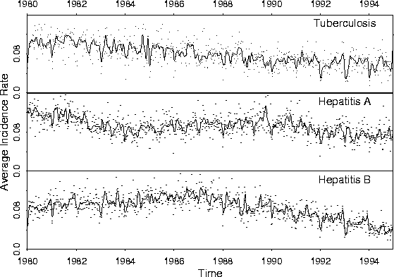
The dataset can be shown as multiple time series for each state and as multiple disease incidence maps for each week. The MIASMA tool is specially designed to explore such data interactively. Here we can only illustrate the overall time trends. Figure 1 shows the weekly average incidence rates (new cases per week per 100,000 people averaged over states) for the 3 diseases. All of the diseases are seasonal and show a nontrivial trend.

**Figure 1:** Behavior of the 3 diseases in the US. Points show average number of new cases each week. Lines are smoothed time series of the points and are shown to emphasize trends.
$\begin{figure} \centerline{\psfig{figure=US.3.new1.ps,width=5.0in,height=3.5in}} \protect \end{figure}$

3. Prediction

The disease incidence rates can be modeled as a smooth function over the territory of the United States and over the time period considered. Of interest is the number of cases of each disease each week in each state. Those quantities represent integrals of the incidence rate function with respect to population density over the territories of individual states and over weeks.

More formally, we are interested in determining a function $f(\mbox{\boldmath${{\bf x}}$ })$ from its integrals $z_i = \int_{A_i} f(\mbox{\boldmath${{\bf x}}$ })dP(\mbox{\boldmath${{\bf x}}$ })$ , where the A_i's are subsets of a finite set $A\subset R^d$ and $dP(\mbox{\boldmath${{\bf x}}$ })$ represents population density. We can model the function as a stochastic process. Let $f(\mbox{\boldmath${{\bf x}}$ })$ be a stochastic process with the index $\mbox{\boldmath${{\bf x}}$ }\in A\subset R^d$ . The z_i are observed integrals of the single realization of f. The simplest predictor for the process fcould then be a piecewise constant function $\hat{f}(\mbox{\boldmath${{\bf x}}$ })$ where

$\begin{displaymath}\hat{f}(\mbox{\boldmath ${{\bf x}}$}) = \sum_i I_{\mbox{\bold... ...A_i} \frac{z_i}{\int_{A_i}1dP(\mbox{\boldmath ${{\bf x}}$})}. \end{displaymath}$

Since we intend to use the predictor in animations, any discontinuity in such a function would be distracting and must be avoided (see Eddy and Mockus 1994). Thus we must consider methods that produce a continuous predictor. In cases when the joint distribution of $(f(\mbox{\boldmath${{\bf x}}$ }),\mbox{\boldmath${{\bf z}}$ })$ is Gaussian, the quantity $E(f(\mbox{\boldmath${{\bf x}}$ })\vert\mbox{\boldmath${{\bf z}}$ })$ is a well known linear function of $\mbox{\boldmath${{\bf z}}$ }$ given by the formula for the conditional normal distribution. Let $\mu(\mbox{\boldmath${{\bf x}}$ }) = E(f(\mbox{\boldmath${{\bf x}}$ }))$ be the mean of the process, $\mu_i = E(z_i)$ be the means of the observed integrals, $c_i(\mbox{\boldmath${{\bf x}}$ })= {\rm Cov}(f(\mbox{\boldmath${{\bf x}}$ }), z_i)$ , and $c_{ij}={\rm Cov}(z_i,z_j)$ . Then

$\begin{displaymath}E(f(\mbox{\boldmath${{\bf x}}$ })\vert\mbox{\boldmath${{\bf z... ...bf x}))(c_{ij})^{-1}((\mu_i) - \mbox{\boldmath${{\bf z}}$ }), \end{displaymath}$

(1)

where $(\mu_i)$ denotes the vector of all $\mu_i$ 's, and $(c_i(\cdot))$ denotes the vector of all c_i's, and (c_ij) is the covariance matrix. In non-Gaussian cases when we know only the first two moments of the vector $(f(\mbox{\boldmath${{\bf x}}$ }),\mbox{\boldmath${{\bf z}}$ })$ , Equation (1) defines the best linear unbiased predictor for $f(\mbox{\boldmath${{\bf x}}$ })$ . Equation (1) is a simple form of equations used in spatial prediction and is referred to as the kriging equation (see, for example, Cressie 1991).

Equation (1) involves quantities $\mu(\cdot), \mu_i, c_i(\cdot)$ and c_ij that are unknown. In space-time prediction we assume the trend $\mu(\cdot)$ to be a constant in spatial dimensions (a constant which varies over time), and we can estimate c_i(s), c_ij as described in Section 4.

4. Dependence Structure

The next step is to estimate geographic and time dependence structure for the stochastic process of disease incidence rates. There are a number of techniques for estimating mean and covariance functions from observations representing point values of a process (see, for example, Delfner 1976, Kitanidis 1983, Cressie 1985, Marshall and Mardia 1985).

In our case the observations are in the form of integrals of the process f described in Section 3. Surprisingly, the estimation of the covariance function of a continuous process from integral observations has not previously been investigated. To illustrate our method we assume that the process f is zero-mean and stationary. We are interested in the covariance function $\gamma(\mbox{\boldmath${{\bf x}}$ }_1-\mbox{\boldmath${{\bf x}}$ }_2)$ of the process f. It should be noted that the symbol $\gamma$ sometimes is used to denote the semi-variogram, e.g. Cressie (1993), but here we use the symbol to denote a covariance function. We obtain the estimate of $\gamma$ by solving appropriate integral equations (a general statistical perspective on solving integral equations can be found in O'Sullivan 1986).

We will describe an efficient algorithm to estimate $\gamma$ , when $\gamma$ is an isotropic covariance function, (isotropic means that $\gamma(\mbox{\boldmath${{\bf x}}$ }_1-\mbox{\boldmath${{\bf x}}$ }_2)$ is a function of only $\Vert\mbox{\boldmath${{\bf x}}$ }_1-\mbox{\boldmath${{\bf x}}$ }_2\Vert$ , where $\Vert\cdot\Vert$ is Euclidean distance), and each A_i is a polygon, or a prism with a polygon base.

In Subsection 4.1 integral equations are obtained for a covariance function. The method used to estimate the covariance function from those equations is then presented. Two main obstacles to an efficient numeric solution are the large number of equations and that the solution must be in the space of positive definite functions. The second problem arises because we want our solution to be a valid covariance function. We address the first problem by designing a fast algorithm to compute the integral of interest and the second problem by re-expressing the isotropic covariance function in terms of a nondecreasing function.

4.1 Estimation Equations

$\begin{eqnarray*}{\rm Cov} (z_i, z_j) = \int_{\mbox{\boldmath${{\bf u}}$ }\in A_... ...(\mbox{\boldmath${{\bf u}}$ }) dP(\mbox{\boldmath${{\bf v}}$ }). \end{eqnarray*}$

The products z_i z_j approximate the integrals $\int_{A_i}\int_{A_j} \gamma (\mbox{\boldmath${{\bf u}}$ }-\mbox{\boldmath${{\bf v}}$ })dP(\mbox{\boldmath${{\bf u}}$ }) dP(\mbox{\boldmath${{\bf v}}$ })$ . (For a stationary process, $\gamma(\mbox{\boldmath${{\bf u}}$ },\mbox{\boldmath${{\bf v}}$ })$ is a function of only $\mbox{\boldmath${{\bf u}}$ }-\mbox{\boldmath${{\bf v}}$ }$ ). We can estimate $\gamma$ by solving an inverse problem for $\gamma$ :

$\begin{displaymath}z_i z_j = \int_{\mbox{\boldmath${{\bf u}}$ }\in A_i}\int_{\mb... ...f u}}$ }) dP(\mbox{\boldmath${{\bf v}}$ }), \; i,j=1,\dots,N. \end{displaymath}$

(2)

In the special case when the A_i's are regularly spaced, the appropriate z_iz_j could be averaged, reducing the number of equations. However, in the general case, it is not clear how to reduce the total number of N(N+1)/2 equations.

For an isotropic and stationary process, $\gamma(\mbox{\boldmath${{\bf u}}$ },\mbox{\boldmath${{\bf v}}$ }) = \gamma (\Vert\mbox{\boldmath${{\bf u}}$ }-\mbox{\boldmath${{\bf v}}$ }\Vert)$ , where $\Vert\cdot\Vert$ is Euclidean distance, and thus Equation (2) can be rewritten as

z_i z_j	=	$\displaystyle \int_{\mbox{\boldmath${{\bf u}}$ }\in A_i}\int_{\mbox{\boldmath${... ...f v}}$ }\Vert)dP(\mbox{\boldmath${{\bf u}}$ }) dP(\mbox{\boldmath${{\bf v}}$ })$
	=	$\displaystyle \int_0^\infty W_{A_iA_j}(l) \gamma (l)dl,$	(3)

where $l=\Vert\mbox{\boldmath${{\bf u}}$ }-\mbox{\boldmath${{\bf v}}$ }\Vert$ and

$\begin{displaymath}W_{A_iA_j}(l) = \int_{\mbox{\boldmath ${{\bf u}}$},\mbox{\bol... ...mbox{\boldmath ${{\bf u}}$}) dP(\mbox{\boldmath ${{\bf v}}$}). \end{displaymath}$

There are two important difficulties when trying to solve Equation (3) with respect to $\gamma$ :

To address the first problem we use a fast algorithm to compute the kernel function W_{A_iA_j}(l). An efficient algorithm to calculate the kernels W_{A_iA_j} is described by Mockus (1994) for cases when the regions A_i are piecewise polygons in R² or prisms with a piecewise polygon base in R³.

To address the second problem we may use a parametric family of covariance functions (e.g., $\gamma (l) = \sigma e^{\alpha l}$ ). Another approach is to re-express the covariance function in terms of some simpler function. A form of an isotropic covariance function for dimension $d\geq 2$ is

$\displaystyle r(l) = \sigma \left(G(0) + \int_0^\infty \phi_Y(ls)dG(s)\right),$			(4)
$\displaystyle \phi_Y (l) = \frac{d-2}{2}{\Huge !} \left(\frac{2}{l}\right)^{\frac{d-2}{2}} J_\frac{d-2}{2}(l),$

where G is a distribution function, $J_\frac{d-2}{2}(l)$ is the Bessel function of the first kind, $\sigma=\gamma(0)$ , lrepresents distance, and s is a scale factor. The isotropic covariance function is a scale mixture of Bessel functions, and the estimation of such a function could be done by estimating the function G appearing in Equation (4).

$\displaystyle {z_i z_j = \int_0^\infty W_{A_iA_j}(l) \gamma (l)dl}$
	=	$\displaystyle { \int_0^\infty W_{A_iA_j}(l) \sigma \left(G(0) + \int_0^\infty \phi_Y(ls)dG(s)\right) dl}$
	=	$\displaystyle \int_0^\infty Q_{A_iA_j}(s) dG(s),$

$\begin{displaymath}Q_{A_iA_j}(s) = \sigma\left(\int_0^\infty W_{A_iA_j}(l) \phi_Y(ls) dl + S_{A_i}S_{A_j}G(0)\right),\end{displaymath}$

and $S_{A_i} = \int_{\mbox{\boldmath${{\bf u}}$ }\in A_i}dP(\mbox{\boldmath${{\bf u}}$ })$ . To simplify the notation the subscript _{A_iA_j} will become simply _ij in the remainder of the paper.

We can look for solutions that minimize the criteria in the following Equations:

$\displaystyle \hat{\gamma} = \arg\min_{{\gamma}} \sum_{i, j} C_{ij}\left\vert z_iz_j -\int W_{ij}(l) \gamma(l)dl\right\vert^p,$			(5)
$\displaystyle \hat{G} = \arg\min_{G} \sum_{i, j} C_{ij}\left\vert z_iz_j - \int Q_{ij}(s) dG(s)\right\vert^p,$			(6)

where C_ij are weights and p > 0. When p=2 the above criteria give a weighted least squares (WLS) solution. Alternative criteria such as maximization of the likelihood function or of the posterior probability would lead to a more complicated set of equations. We chose to solve the simplest Equations (5) and (6).

4.2 Solving Integral Equations

In this section we discuss the ways to construct an estimate of the covariance function. When p=2 the optimality criteria in the equations above are quadratic in $\gamma (\cdot)$ and dG. Hence, the unconstrained solutions are linear functions (functionals) of the data (z_iz_j). Unfortunately, the constraints require that $\gamma$ be a covariance function and G be a nondecreasing function. To simplify the optimization problem we can perform estimation in two steps: first we do an unconstrained minimization (simple least squares problem), and then we project the solution into the desired space. However, the final estimate after the projection may be suboptimal. Another approach (used in the examples of the next section) is to perform optimization entirely within the restricted domain. In that case we have to use nonlinear minimization techniques (see Appendix).

In the following examples we solve Equation (5) for $\gamma$ of a parametric form, i.e., $\gamma(l) = \sigma \exp (\alpha l)$ . In solving Equation (6) it is convenient to represent G as the sum of an absolutely continuous function g and a step function. Then the integral in (6) can be rewritten as $\int Q_{ij}(s) dG(s) = \int Q_{ij}(s)g(s)ds + \sum_{k=1,\dots,N} G_k\int_{S_k}^\infty Q_{ij}(s)ds$ , where G_k=G(S_k)-G(S_k-) are jump sizes and S_k are jump locations. In this form we have the simplest constraints on the parameters ( $g(s)\geq 0, G_k\geq 0$ ). Since the number of observations z_i is finite, the solutions $\gamma (\cdot)$ and $G(\cdot)$ are not well defined unless we estimate parameterized versions of those functions or add regularization/penalty terms to achieve a unique solution.

4.3 Example

4.3.1 Generated data

To illustrate the behavior of the covariances between regions, we first consider an example with simulated data and the covariance function $\gamma (l) = \sigma \int_0^\infty J_0(ls)dG(s) = \sigma J_0(10l)$ , where

and J₀ is a Bessel function of the first kind. The constant 10 gives approximately two periods for the covariance function (see Figure 2). A smaller value of the constant would lead to fewer oscillations. The 48 regions $A_1, \dots, A_{48}$ partition the map of United States into the 48 contiguous states. The map obtained from statlib (http://lib.stat.cmu.edu/maps/) was converted to Albers equal area projection coordinates, (see Deetz and Adams 1921.) These coordinates were rescaled so that the area of the map would be equal to 1. All distances in this paper were obtained in that way. Thus, for example, on our scale a distance of 3000 miles is approximately 1.

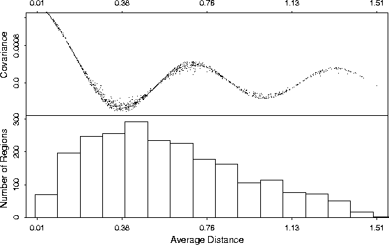
Figure 2 shows exact covariances ( $\int_{u\in A_i}\int_{v\in A_j} \gamma(u-v)dudv$ ) between all possible pairs of regions. The covariances are plotted on the Y axis, while the average distances between regions are plotted on the X axis; average distance d_ij between regions A_i, A_j is given by

$\begin{displaymath}d_{ij} = \frac{\int_0^\infty W_{ij}(l) l dl}{\int_0^\infty W_{ij}(l) dl}.\end{displaymath}$

There are 48 (48+1)/2= 1176 points in the plot. The points approximately follow the line of $\gamma (l)$ .

**Figure 2:** Exact Covariances. Plot of covariances versus average distance is in the top panel and the histogram of average distances is in the bottom panel.
$\begin{figure} \centerline{\psfig{figure=covariances1.ps,width=5.0in,height=3.2in}} \protect \end{figure}$

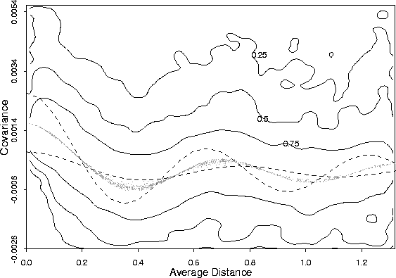
The display and assessment of the variability of quantities (z_iz_j) used to estimate the covariance function are given in Figure 3. Figure 3 shows the estimated conditional density d(x, y | x) of observed covariances between all possible pairs of regions, where x is the average distance between regions and y is the covariance between regions. The density was estimated empirically by generating 1000 realizations of the process f. To reduce the variance we calculated one hundred 10 point averages $\sum_{k=1}^{10}\frac{z^k_iz^k_j}{10}$ , where $z^k_i = \int_{A_i}f(x)dx$ are integrals of the realization k of the process f over region A_i. The two dimensional density d(x, y)and the marginal density d(x) were estimated using David Scott's ash package available from statlib ( http://lib.stat.cmu.edu). The contour level lines of $\frac{d(x, y)}{d(x)}$ displayed in Figure 3 approximate highest density regions having probabilities 0.75, 0.50, and 0.25.

**Figure 3:** Estimated conditional density. The solid lines are contours of highest conditional density d(x, y |x), the dots are exact covariances, and the dashed lines are two covariance functions based on the extreme values of the estimated parameters.
$\begin{figure} \par\centerline{\psfig{figure=newObsCovariances1.ps,width=5.0in,height=3.5in}} \protect \end{figure}$

We then estimated the covariance function $\gamma(l) = \sigma J_0(\alpha l)$ from the same data obtaining 100 estimates of $\alpha$ and $\sigma$ by solving Equation (6) with $C_{ij} = 1, \; p= 1,$ and p=2. The results are shown in Table 2. The least squares solution (p=2) overestimates the scale parameter and is much less stable than the solution for p=1. Therefore we used p=1 in the next section. The scale parameter overestimation would have no effect on the mean of the predictor (Equation 1) but would entail larger error bounds. Two covariance functions shown in Figure 3 are based on the extreme estimated parameters for p=1 ( $\alpha_1=9.1, \sigma_1=0.41$ and $\alpha_2=10.9, \sigma_2=1.63$ ). The covariance function corresponding to the median of estimated parameters is not shown since it obscures the exact covariances.

**Table 2:** Quantiles of Estimated Parameters Based on 100 Estimates.
	Parameter	Quantiles
		0	0.25	0.50	0.75	1
p=2	$\alpha$	5.4	9.7	11	22.8	1056
p=2	$\sigma$	0.58	1.87	2.54	5.5	615
p=1	$\alpha$	9.1	9.8	10	10.2	10.9
p=1	$\sigma$	0.41	0.76	0.9	1.63	1.63

NOTE: The parameters used to generate the data were $\alpha = 10,\; \sigma = 1$ .

4.3.2 Disease data

The incidence rate process of disease data often has seasonal and longer time trends (see Figure 1) that need to be removed before estimation of the covariance function. The data are based on reports by state epidemiologists, who themselves receive reports from a variety of sources, such as individual practitioners, hospitals, laboratories, and health departments. Hence each state might have a slightly different disease reporting mechanism.

Let z_ij be the reported incidence rate in state i for time interval j. Very good temporal resolution (weeks) and poor spatial resolution (states) lead to strong temporal and weaker spatial correlations. To increase spatial correlations we aggregated the data into periods of four weeks, so j corresponds to approximately one month.

Trends were removed by fitting state effects s_i and time effects t_j via median polish (Mosteller and Tukey (1983)) implemented as twoway function in S language (Becker, et al (1988)). The residuals

for any particular state did not have an obvious trend. The residuals were normalized since we were comparing the shapes of the covariance functions, not the scales (the minimization criteria are scale invariant, hence the actual covariance function can be obtained by multiplying the estimated covariance function by the square of the normalization factor).

To illustrate the behavior of observed covariances for temporal lags l=0, 3, 6, Figure 4 shows three quantiles (25, 50, and 75) for the average lagged covariance computed over equally spaced intervals (0-0.1, 0.1-0.2, ...). For each interval [x_i,x_i+1) the average observed lagged covariances $\zeta_{i,k} (l) = \sum_{j=1, N-l}(\eta_{i,j}, \eta_{k, j+l})/(N-l)$ were computed between regions having distance in the range of [x_i,x_i+1), and the three quantiles were calculated.

Estimated covariance functions are also shown in Figure 4 and Table 3. We used $\zeta_{i,k}(l), l=0, 3, 6$ to estimate parameters $\alpha, \sigma$ for the covariance functions $\gamma_e(l) = \sigma e^{-\alpha l}$ and $\gamma_b(l) = \sigma J_0(\alpha l)$ by solving Equations (5, 6) with C_ij = 1and p=1. The population density dP in Equation (3) was assumed constant over the territory of each state. More precise definition of W_ij's would be obtained using smaller regions like counties or census tracts.

Judging by the estimated parameters (Table 3) of the exponential covariance function, the Tuberculosis data has short range correlations rapidly decreasing with geographic distance, unlike the other two diseases. The quantiles in Figure 4 indicate that for Hepatitis B, which spreads by a different mechanism than other diseases (contaminated blood products), covariances appear to increase for the largest distances, possibly showing relationship between large cities on east and west coasts.

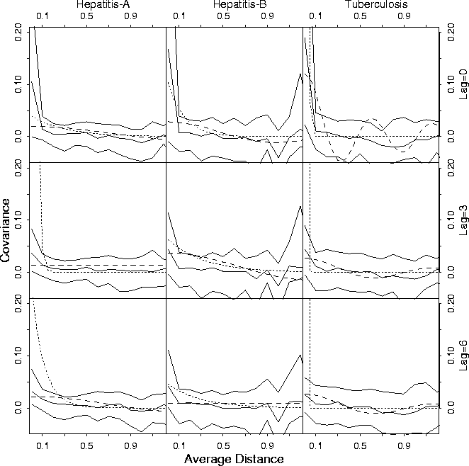**Figure:** Behavior of two estimated covariance functions. The dotted line is $\gamma _e$ , the dashed line is $\gamma _b$ , and the solid lines are the three quantiles of the observed covariances (25, 50, and 75).
$\begin{figure} \centerline{\psfig{figure=lagCov2.1.ps,width=6.0in,height=6in}} \protect \end{figure}$

The exponential covariance model did not fit the observed covariances very well because at geographic distances equal to 2000 miles, covariances for all three diseases appear to be negative. Table 3 shows the cyclic covariance function outperformed the exponential covariance function in 6 out of 9 cases. The large peak at zero (no temporal lag) for the Tuberculosis data caused excessive oscillations for the cyclic covariance function. This example suggests that a weighted mixture of exponential and Bessel functions might best describe Tuberculosis data.

**Table:** Estimated Shape Parameter ( $\alpha$ ) for Two Covariance Functions.
function	Disease	Lag 0	Lag 3	Lag 6
$\gamma _e$	Hepatitis A	3.18	45	8.9+
$\gamma _b$	Hepatitis A	2.52+	.002+	2.58
$\gamma _e$	Hepatitis B	6.7	3.0	3.3+
$\gamma _b$	Hepatitis B	3.93+	2.9+	.02
$\gamma _e$	Tuberculosis	157	271+	672
$\gamma _b$	Tuberculosis	11.5+	6.11	5.9+

5. Discussion and Summary

We designed and implemented a set of methods to estimate the dependence structure of a spatial-temporal stochastic process when the available data are represented in the form of integrals of the considered process. We illustrated our techniques on simulated data and applied them to real data concerning the spread of three diseases. We concentrated on spatial (two-dimensional) isotropic covariance functions and estimated two parametric forms of the covariance function. We described a way to re-express a covariance function as a nonnegative function for the purpose of numeric non-parametric estimation.

Our estimation method was based on a solution to a system of integral equations given in Equation (2) via numeric optimization. In simulated data we were able to recover the original covariance function. In real data concerning infectious diseases we obtained spatial correlations that reasonably describe possible mechanisms by which each disease spreads. We, therefore, achieved our purpose of obtaining a quantitative estimate of variability and smoothness for the predictor of a stochastic process. This makes possible prediction of spatial and space-time processes using observations representing averages of such process.

The shapes and locations of the regions affect the quality of the estimate at various spatial distances. If the goal of the estimation is to obtain a reliable covariance function estimate at a particular distance l it is best to have more pairs of small regions that have average distance close to l. To obtain the estimate for all distances it is better to have regions of different sizes and shapes (for more discussion see Mockus 1994).

There still are a number of issues with the described approach in general and with the treatment of the disease data in particular. The approach assumes an isotropic covariance function (in two spatial dimensions). The numeric optimization required to achieve the estimates reliably is nontrivial (see Appendix). Simple covariance functions were used in the examples; use of covariance function with larger number of parameters would make the optimization task even harder. The temporal trends of the diseases were removed using simple median polish and the spatial covariance function was fitted independently for different time lags. A more sophisticated approach would be to fit a time series model (like ARMA) together with spatial covariances.