


 |
 |
 |
 |
 |
 |
 |
A heap is a special kind of tree that happens to be an efficient implementation of a priority queue. This figure shows the relationships among the data structures in this chapter.
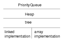
Ordinarily we try to maintain as much distance as possible between an ADT and its implementation, but in the case of the Heap, this barrier breaks down a little. The reason is that we are interested in the performance of the operations we implement. For each implementation there are some operations that are easy to implement and efficient, and others that are clumsy and slow.
It turns out that the array implementation of a tree works particularly well as an implementation of a Heap. The operations the array performs well are exactly the operations we need to implement a Heap.
To understand this relationship, we will proceed in a few steps. First, we need to develop ways of comparing the performance of various implementations. Next, we will look at the operations Heaps perform. Finally, we will compare the Heap implementation of a Priority Queue to the others (arrays and lists) and see why the Heap is considered particularly efficient.
When we compare algorithms, we would like to have a way to tell when one is faster than another, or takes less space, or uses less of some other resource. It is hard to answer those questions in detail, because the time and space used by an algorithm depend on the implementation of the algorithm, the particular problem being solved, and the hardware the program runs on.
The objective of this section is to develop a way of talking about performance that is independent of all of those things, and only depends on the algorithm itself. To start, we will focus on run time; later we will talk about other resources.
Our decisions are guided by a series of constraints:
To make this process more concrete, consider two algorithms we have already seen for sorting an array of integers. The first is selection sort, which we saw in Section 13.7. Here is the pseudocode we used there.
void selectionsort (vector<card> array) {To perform the operations specified in the pseudocode, we wrote helper methods named findLowest() and swap. In pseudocode, findLowest() looks like this
// find the index of the lowest item betweenAnd swap looks like this:
void swap (int& i, int& j) {To analyze the performance of this algorithm, the first step is to decide what operations to count. Obviously, the program does a lot of things: it increments i, compares it to the length of the deck, it searches for the largest element of the array, etc. It is not obvious what the right thing is to count.
It turns out that a good choice is the number of times we compare two items. Many other choices would yield the same result in the end, but this is easy to do and we will find that it allows us to compare most easily with other sort algorithms.
The next step is to define the "problem size." In this case it is natural to choose the size of the array, which we'll call n.
Finally, we would like to derive an expression that tells us how many abstract operations (specifically, comparisons) we have to do, as a function of n.
We start by analyzing the helper methods. swap copies several references, but it doesn't perform any comparisons, so we ignore the time spent performing swaps. findLowest starts at i and traverses the array, comparing each item to lowest. The number of items we look at is n-i, so the total number of comparisons is n-i-1.
Next we consider how many times findLowest gets invoked and what the value of i is each time. The last time it is invoked, i is n-2 so the number of comparisons is 1. The previous iteration performs 2 comparisons, and so on. During the first iteration, i is 0 and the number of comparisons is n-1.
So the total number of comparisons is 1 + 2 + ��� + n-1. This sum is equal to n2/2 - n/2. To describe this algorithm, we would typically ignore the lower order term (n/2) and say that the total amount of work is proportional to n2. Since the leading order term is quadratic, we might also say that this algorithm is quadratic time.
In Section 13.10 I claimed that mergesort takes time that is proportional to n log n, but I didn't explain how or why. Now I will.
Again, we start by looking at pseudocode for the algorithm. For mergesort, it's
vector<Card> mergeSort (vector<Card> array) {At each level of the recursion, we split the array in half, make two recursive calls, and then merge the halves. Graphically, the process looks like this:

Each line in the diagram is a level of the recursion. At the top, a single array divides into two halves. At the bottom, n arrays (with one element each) are merged into n/2 arrays (with 2 elements each).
The first two columns of the table show the number of arrays at each level and the number of items in each array. The third column shows the number of merges that take place at each level of recursion. The next column is the one that takes the most thought: it shows the number of comparisons each merge performs.
If you look at the pseudocode (or your implementation) of merge, you should convince yourself that in the worst case it takes m-1 comparisons, where m is the total number items being merged.
The next step is to multiply the number of merges at each level by the amount of work (comparisons) per merge. The result is the total work at each level. At this point we take advantage of a small trick. We know that in the end we are only interested in the leading-order term in the result, so we can go ahead and ignore the -1 term in the comparisons per merge. If we do that, then the total work at each level is simply n.
Next we need to know the number of levels as a function of n. Well, we start with an array of n items and divide it in half until it gets to 1. That's the same as starting at 1 and multiplying by 2 until we get to n. In other words, we want to know how many times we have to multiply 2 by itself before we get to n. The answer is that the number of levels, l, is the logarithm, base 2, of n.
Finally, we multiply the amount of work per level, n, by the number of levels, log2 n to get n log2 n, as promised. There isn't a good name for this functional form; most of the time people just say, "en log en."
It might not be obvious at first that n log2 n is better than n2, but for large values of n, it is. As an exercise, write a program that prints n log2 n and n2 for a range of values of n.
Performance analysis takes a lot of handwaving. First we ignored most of the operations the program performs and counted only comparisons. Then we decided to consider only worst case performance. During the analysis we took the liberty of rounding a few things off, and when we finished, we casually discarded the lower-order terms.
When we interpret the results of this analysis, we have to keep all this hand-waving in mind. Because mergesort is n log2 n, we consider it a better algorithm than selection sort, but that doesn't mean that mergesort is always faster. It just means that eventually, if we sort bigger and bigger arrays, mergesort will win.
How long that takes depends on the details of the implementation, including the additional work, besides the comparisons we counted, that each algorithm performs. This extra work is sometimes called overhead. It doesn't affect the performance analysis, but it does affect the run time of the algorithm.
For example, our implementation of mergesort actually allocates subarrays before making the recursive calls and then lets them get garbage collected after they are merged. Looking again at the diagram of mergesort, we can see that the total amount of space that gets allocated is proportional to n log2 n, and the total number of objects that get allocated is about 2n. All that allocating takes time.
Even so, it is most often true that a bad implementation of a good algorithm is better than a good implementation of a bad algorithm. The reason is that for large values of n the good algorithm is better and for small values of n it doesn't matter because both algorithms are good enough.
As an exercise, write a program that prints values of 1000 n log2 n and n2 for a range of values of n. For what value of n are they equal?
In Chapter 20 we looked at an implementation of a Priority Queue based on an array. The items in the array are unsorted, so it is easy to add a new item (at the end), but harder to remove an item, because we have to search for the item with the highest priority.
An alternative is an implementation based on a sorted list. In this case when we insert a new item we traverse the list and put the new item in the right spot. This implementation takes advantage of a property of lists, which is that it is easy to insert a new node into the middle. Similarly, removing the item with the highest priority is easy, provided that we keep it at the beginning of the list.
Performance analysis of these operations is straightforward. Adding an item to the end of an array or removing a node from the beginning of a list takes the same amount of time regardless of the number of items. So both operations are constant time.
Any time we traverse an array or list, performing a constant-time operation on each element, the run time is proportional to the number of items. Thus, removing something from the array and adding something to the list are both linear time.
So how long does it take to insert and then remove n items from a Priority Queue? For the array implementation, n insertions takes time proportional to n, but the removals take longer. The first removal has to traverse all n items; the second has to traverse n-1, and so on, until the last removal, which only has to look at 1 item. Thus, the total time is 1 + 2 + ��� + n, which is (still) n2/2 - n/2. So the total for the insertions and the removals is the sum of a linear function and a quadratic function. The leading term of the result is quadratic.
The analysis of the list implementation is similar. The first insertion doesn't require any traversal, but after that we have to traverse at least part of the list each time we insert a new item. In general we don't know how much of the list we will have to traverse, since it depends on the data and what order they are inserted, but we can assume that on average we have to traverse half of the list. Unfortunately, even traversing half of the list is still a linear operation.
So, once again, to insert and remove n items takes time proportional to n2. Thus, based on this analysis we cannot say which implementation is better; both the array and the list yield quadratic run times.
If we implement a Priority Queue using a heap, we can perform both insertions and removals in time proportional to log n. Thus the total time for n items is n log n, which is better than n2. That's why, at the beginning of the chapter, I said that a heap is a particularly efficient implementation of a Priority Queue.
A heap is a special kind of tree. It has two properties that are not generally true for other trees:
Both of these properties bear a little explaining. This figure shows a number of trees that are considered complete or not complete:
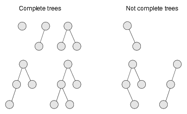
An empty tree is also considered complete. We can define completeness more rigorously by comparing the height of the subtrees. Recall that the height of a tree is the number of levels.
Starting at the root, if the tree is complete, then the height of the left subtree and the height of the right subtree should be equal, or the left subtree may be taller by one. In any other case, the tree cannot be complete.
Furthermore, if the tree is complete, then the height relationship between the subtrees has to be true for every node in the tree.
It is natural to write these rules as a recursive function:
int height(Tree* head)For this example I used the linked implementation of a tree. As an exercise, write the same function for the array implementation. Also as an exercise, write the height function. The height of a NULL tree is 0 and the height of a leaf node is 1.
The heap property is similarly recursive. In order for a tree to be a heap, the largest value in the tree has to be at the root, and the same has to be true for each subtree. As another exercise, write a function that checks whether a tree has the heap property.
It might seem odd that we are going to remove things from the heap before we insert any, but I think removal is easier to explain.
At first glance, we might think that removing an item from the heap is a constant time operation, since the item with the highest priority is always at the root. The problem is that once we remove the root node, we are left with something that is no longer a heap. Before we can return the result, we have to restore the heap property. We call this operation reheapify.
The situation is shown in the following figure:
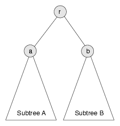
The root node has priority r and two subtrees, A and B. The value at the root of Subtree A is a and the value at the root of Subtree B is b.
We assume that before we remove r from the tree, the tree is a heap. That implies that r is the largest value in the heap and that a and b are the largest values in their respective subtrees.
Once we remove r, we have to make the resulting tree a heap again. In other words we need to make sure it has the properties of completeness and heapness.
The best way to ensure completeness is to remove the bottom-most, right-most node, which we'll call c and put its value at the root. In a general tree implementation, we would have to traverse the tree to find this node, but in the array implementation, we can find it in constant time because it is always the last (non-null) element of the array.
Of course, the chances are that the last value is not the highest, so putting it at the root breaks the heapness property. Fortunately it is easy to restore. We know that the largest value in the heap is either a or b. Therefore we can select whichever is larger and swap it with the value at the root.
Arbitrarily, let's say that b is larger. Since we know it is the highest value left in the heap, we can put it at the root and put c at the top of Subtree B. Now the situation looks like this:
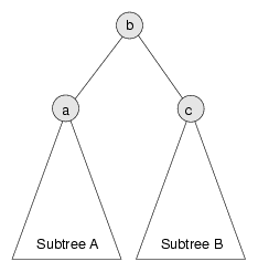
Again, c is the value we copied from the last entry in the array and b is the highest value left in the heap. Since we haven't changed Subtree A at all, we know that it is still a heap. The only problem is that we don't know if Subtree B is a heap, since we just stuck a (probably low) value at its root.
Wouldn't it be nice if we had a method that could reheapify Subtree B? Wait... we do!
Inserting a new item in a heap is a similar operation, except that instead of trickling a value down from the top, we trickle it up from the bottom.
Again, to guarantee completeness, we add the new element at the bottom-most, rightmost position in the tree, which is the next available space in the array.
Then to restore the heap property, we compare the new value with its neighbors. The situation looks like this:
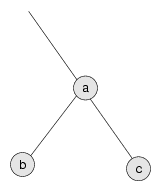
The new value is c. We can restore the heap property of this subtree by comparing c to a. If c is smaller, then the heap property is satisfied. If c is larger, then we swap c and a. The swap satisfies the heap property because we know that c must also be bigger than b, because c > a and a > b.
Now that the subtree is reheapified, we can work our way up the tree until we reach the root.
For both insert and remove, we perform a constant time operation to do the actual insertion and removal, but then we have to reheapify the tree. In one case we start at the root and work our way down, comparing items and then recursively reheapifying one of the subtrees. In the other case we start at a leaf and work our way up, again comparing elements at each level of the tree.
As usual, there are several operations we might want to count, like comparisons and swaps. Either choice would work; the real issue is the number of levels of the tree we examine and how much work we do at each level. In both cases we keep examining levels of the tree until we restore the heap property, which means we might only visit one, or in the worst case we might have to visit them all. Let's consider the worst case.
At each level, we perform only constant time operations like comparisons and swaps. So the total amount of work is proportional to the number of levels in the tree, a.k.a. the height.
So we might say that these operations are linear with respect to the height of the tree, but the "problem size" we are interested in is not height, it's the number of items in the heap.
As a function of n, the height of the tree is log2 n. This is not true for all trees, but it is true for complete trees. To see why, think of the number of nodes on each level of the tree. The first level contains 1, the second contains 2, the third contains 4, and so on. The ith level contains 2i nodes, and the total number in all levels up to i is 2i - 1. In other words, 2h = n, which means that h = log2 n.
Thus, both insertion and removal take logarithmic time. To insert and remove n items takes time proportional to n log2 n.
The result of the previous section suggests yet another algorithm for sorting. Given n items, we insert them into a Heap and then remove them. Because of the Heap semantics, they come out in order. We have already shown that this algorithm, which is called heapsort, takes time proportional to n log2 n, which is better than selection sort and the same as mergesort.
As the value of n gets large, we expect heapsort to be faster than selection sort, but performance analysis gives us no way to know whether it will be faster than mergesort. We would say that the two algorithms have the same order of growth because they grow with the same functional form. Another way to say the same thing is that they belong to the same complexity class.
Complexity classes are sometimes written in "big-O notation". For example, O(n2), pronounced "oh of en squared" is the set of all functions that grow no faster than n2 for large values of n. To say that an algorithm is O(n2) is the same as saying that it is quadratic. The other complexity classes we have seen, in decreasing order of performance, are:
| O(1) | constant time |
| O(log n) | logarithmic |
| O(n) | linear |
| O(n log n) | "en log en" |
| O(n2) | quadratic |
| O(2n) | exponential |
So far none of the algorithms we have looked at are exponential. For large values of n, these algorithms quickly become impractical. Nevertheless, the phrase "exponential growth" appears frequently in even non-technical language. It is frequently misused so I wanted to include its technical meaning.
People often use "exponential" to describe any curve that is increasing and accelerating (that is, one that has positive slope and curvature). Of course, there are many other curves that fit this description, including quadratic functions (and higher-order polynomials) and even functions as undramatic as n log n. Most of these curves do not have the (often detrimental) explosive behavior of exponentials.
As an exercise, compare the behavior of 1000 n2 and 2n as the value of n increases.
Revised 2008-12-13.
 |
 |
 |
 |
 |
 |
 |